Understanding Face Detection via AdaBoost - CSE 455.1
Face detection using AdaBoost algorithm involves training a sequence of weak classifiers to form a strong final classifier. The process includes weighted data sampling, modifying AdaBoost for Viola-Jones face detector features, and more. Face detection and recognition technology is advancing rapidly, as demonstrated by state-of-the-art demos like Viola-Jones face detection. Boosting techniques like AdaBoost work by iteratively updating weights for each training example to improve classification accuracy.

Download Presentation

Please find below an Image/Link to download the presentation.
The content on the website is provided AS IS for your information and personal use only. It may not be sold, licensed, or shared on other websites without obtaining consent from the author. Download presentation by click this link. If you encounter any issues during the download, it is possible that the publisher has removed the file from their server.
E N D
Presentation Transcript
Recognition Part II: Face Detection via AdaBoost Linda Shapiro CSE 455 1
Whats Coming 1. The basic AdaBoost algorithm (next) 2. The Viola Jones face detector features 3. The modified AdaBoost algorithm that is used in Viola-Jones face detection 4. HW 4 2
Learning from weighted data sample class weight 1.5 2.6 I 1/2 2.3 8.9 II 1/2 Consider a weighted dataset D(i) weight of ith training example (xi,yi) Interpretations: ith training example counts as if it occurred D(i) times If I were to resample data, I would get more samples of heavier data points Now, always do weighted calculations: e.g., MLE for Na ve Bayes, redefine Count(Y=y) to be weighted count: where (P) = 1 when P is true else 0, and setting D(j)=1 (or any constant like 1/n) for all j, will recreates unweighted case 3
AdaBoost Overview Input is a set of training examples (Xi, yi) i = 1 to m. We are going to train a sequence of weak classifiers, such as decision trees, neural nets or SVMs. Weak because not as strong as the final classifier. The training examples will have weights, initially all equal. At each step, we use the current weights, train a new classifier, and use its performance on the training data to produce new weights for the next step. But we keep ALL the weak classifiers. When it s time for testing on a new feature vector, we will combine the results from all of the weak classifiers. 4
Idea of Boosting (from AI text) 5
m samples 2 classes labeled training data start with equal weights How to choose Many possibilities. Will see one shortly! update weights weight at time t+1 for sample i sum over m samples Final Result: linear sum of base or weak classifier outputs. 6
(P) = 1 when P is true else 0 error t is a weight for weak learner ht. 7
Face detection State-of-the-art face detection demo (Courtesy Boris Babenko) 11
Face detection and recognition Detection Recognition Sally 12
Face detection Where are the faces? 13
Face Detection What kind of features? What kind of classifiers? Uses a pyramid to get faces of many different sizes. Neural Net Classifier 14
Image Features +1 -1 Rectangle filters People call them Haar-like features, since similar to 2D Haar wavelets. Value = (pixels in white area) (pixels in black area) 15
Feature extraction Rectangular filters Feature output is difference between adjacent regions Efficiently computable with integral image: any sum can be computed in constant time Avoid scaling images scale features directly for same cost 16 Viola & Jones, CVPR 2001 K. Grauman, B. Leibe
Recall: Sums of rectangular regions 239 240 225 206 185 188 218 211 206 216 225 How do we compute the sum of the pixels in the red box? 243 242 239 218 110 67 31 34 152 213 206 208 221 243 242 123 58 94 82 132 77 108 208 208 215 235 217 115 212 243 236 247 139 91 209 208 211 After some pre-computation, this can be done in constant time for any box. 233 208 131 222 219 226 196 114 74 208 213 214 232 217 131 116 77 150 69 56 52 201 228 223 232 232 182 186 184 179 159 123 93 232 235 235 232 236 201 154 216 133 129 81 175 252 241 240 235 238 230 128 172 138 65 63 234 249 241 245 237 236 247 143 59 78 10 94 255 248 247 251 234 237 245 193 55 33 115 144 213 255 253 251 248 245 161 128 149 109 138 65 47 156 239 255 190 107 39 102 94 73 114 58 17 7 51 137 This trick is commonly used for computing Haar wavelets (a fundemental building block of many object recognition approaches.) 23 32 33 148 168 203 179 43 27 17 12 8 17 26 12 160 255 255 109 22 26 19 35 24
Sums of rectangular regions The trick is to compute an integral image. Every pixel is the sum of its neighbors to the upper left. Sequentially compute using:
Sums of rectangular regions Solution is found using: A B A + D B - C What if the position of the box lies between pixels? C D Use bilinear interpolation.
Large library of filters Considering all possible filter parameters: position, scale, and type: 160,000+ possible features associated with each 24 x 24 window Use AdaBoost both to select the informative features and to form the classifier 20 Viola & Jones, CVPR 2001
Feature selection For a 24x24 detection region, the number of possible rectangle features is ~160,000! At test time, it is impractical to evaluate the entire feature set Can we create a good classifier using just a small subset of all possible features? How to select such a subset? 21
AdaBoost for feature+classifier selection Want to select the single rectangle feature and threshold that best separates positive (faces) and negative (non-faces) training examples, in terms of weighted error. t is a threshold for classifier ht Resulting weak classifier: 0 For next round, reweight the examples according to errors, choose another filter/threshold combo. Outputs of a possible rectangle feature on faces and non-faces. 22 Viola & Jones, CVPR 2001
Weak Classifiers Each weak classifier works on exactly one rectangle feature. Each weak classifier has 3 associated variables 1. its threshold 2. its polarity p 3. its weight The polarity can be 0 or 1 The weak classifier computes its one feature f When the polarity is 1, we want f > for face When the polarity is 0, we want f < for face The weight will be used in the final classification by AdaBoost. The code does not actually compute h. h(x) = 1 if p*f(x) < p , else 0 used for the combination step 23
AdaBoost: Intuition Consider a 2-d feature space with positive and negative examples. Each weak classifier splits the training examples with at least 50% accuracy. Examples misclassified by a previous weak learner are given more emphasis at future rounds. 24 K. Grauman, B. Leibe Figure adapted from Freund and Schapire
AdaBoost: Intuition 25 K. Grauman, B. Leibe
AdaBoost: Intuition Final classifier is combination of the weak classifiers 26 K. Grauman, B. Leibe
t = t / (1- t): the training error of the classifier ht Final classifier is combination of the weak ones, weighted according to error they had. 27
AdaBoost Algorithm modified by Viola Jones NOTE: Our code uses equal weights for all samples {x1, xn} For T rounds: meaning we will construct T weak classifiers Normalize weights Find the best threshold and polarity for each feature, and return error. sum over training samples Re-weight the examples: Incorrectly classified -> more weight Correctly classified -> less weight 28
Recall Classification Nearest Neighbor Na ve Bayes Decision Trees and Forests Logistic Regression Boosting .... Face Detection Simple Features Integral Images Boosting A B C D 29
Picking the (threshold for the) best classifier Efficient single pass approach: At each sample compute: = min ( S + (T S), S + (T S) ) Find the minimum value of , and use the value of the corresponding sample as the threshold. S = sum of samples with feature value below the current sample T = total sum of all samples S and T are for faces; S and T are for background. 30
Picking the threshold for the best classifier The features are actually sorted in the code according to numeric value! Efficient single pass approach: At each sample compute: = min ( S + (T S), S + (T S) ) Find the minimum value of , and use the value of the corresponding sample as the threshold. S = sum of weights of samples with feature value below the current sample T = total sum of all samples S and T are for faces; S and T are for background. 31
Picking the threshold for the best classifier The features for the training samples are actually sorted in the code according to numeric value! Algorithm: 1. find AFS, the sum of the weights of all the face samples 2. find ABG, the sum of the weights of all the background samples 3. set to zero FS, the sum of the weights of face samples so far 4. set to zero BG, the sum of the weights of background samples so far 5. go through each sample s in a loop IN THE SORTED ORDER At each sample, add weight to FS or BG and compute: = min (BG + (AFS FS), FS + (ABG BG)) Find the minimum value of e, and use the feature value of the corresponding sample as the threshold. 32
Whats going on? error = min (BG + (AFS FS), FS + (ABG BG)) left right Let s pretend the weights on the samples are all 1 s. The samples are arranged in a sorted order by feature value and we know which ones are faces (f) and background (b). Left is the number of background patches so far plus the number of faces yet to be encountered. Right is the number of faces so far plus the number of background patches yet to be encountered. 0+5-1 1+5-0 b b b f b f f b f f (6,4) (7,3) (8,2) (7,3) (8,2) (7,3) (4,4) (7,3) (6,4) (5,5) 4 3 2 3 2 3 4 3 4 5 33
Measuring classification performance Confusion matrix Predicted class Class1 Class2 Class3 Accuracy (TP+TN)/ (TP+TN+FP+FN) Class1 40 1 6 Actual class Class2 3 25 7 Class3 4 9 10 True Positive Rate=Recall TP/(TP+FN) False Positive Rate FP/(FP+TN) Precision TP/(TP+FP) F1 Score 2*Recall*Precision/ (Recall+Precision) Predicted Positive Negative Positive True Positive False Negative Actual Negative False Positive True Negative 34
Boosting for face detection First two features selected by boosting: This feature combination can yield 100% detection rate and 50% false positive rate 35
Boosting for face detection A 200-feature classifier can yield 95% detection rate and a false positive rate of 1 in 14084 Is this good enough? 36 Receiver operating characteristic (ROC) curve
Attentional cascade (from Viola-Jones) This part will be extra credit for HW4 We start with simple classifiers which reject many of the negative sub-windows while detecting almost all positive sub-windows Positive response from the first classifier triggers the evaluation of a second (more complex) classifier, and so on A negative outcome at any point leads to the immediate rejection of the sub-window T T T T FACE IMAGE SUB-WINDOW Classifier 2 Classifier 3 Classifier 1 F F F 37 NON-FACE NON-FACE NON-FACE
Attentional cascade Chain of classifiers that are progressively more complex and have lower false positive rates: Receiver operating characteristic % False Pos 0 50 vsfalse neg determined by 0 100 % Detection T T T T FACE IMAGE SUB-WINDOW Classifier 2 Classifier 3 Classifier 1 F F F 38 NON-FACE NON-FACE NON-FACE
Attentional cascade The detection rate and the false positive rate of the cascade are found by multiplying the respective rates of the individual stages A detection rate of 0.9 and a false positive rate on the order of 10-6 can be achieved by a 10-stage cascade if each stage has a detection rate of 0.99 (0.9910 0.9) and a false positive rate of about 0.30 (0.310 6 10-6) T T T T FACE IMAGE SUB-WINDOW Classifier 2 Classifier 3 Classifier 1 F F F 39 NON-FACE NON-FACE NON-FACE
Training the cascade Set target detection and false positive rates for each stage Keep adding features to the current stage until its target rates have been met Need to lower AdaBoost threshold to maximize detection (as opposed to minimizing total classification error) Test on a validation set If the overall false positive rate is not low enough, then add another stage Use false positives from current stage as the negative training examples for the next stage 40
Viola-Jones Face Detector: Summary Train cascade of classifiers with AdaBoost Faces New image Selected features, thresholds, and weights Non-faces Train with 5K positives, 350M negatives Real-time detector using 38 layer cascade 6061 features in final layer [Implementation available in OpenCV: http://www.intel.com/technology/computing/opencv/] 41
The implemented system Training Data 5000 faces All frontal, rescaled to 24x24 pixels 300 million non-faces 9500 non-face images Faces are normalized Scale, translation Many variations Across individuals Illumination Pose 42
System performance Training time: weeks on 466 MHz Sun workstation 38 layers, total of 6061 features Average of 10 features evaluated per window on test set On a 700 Mhz Pentium III processor, the face detector can process a 384 by 288 pixel image in about .067 seconds 15 Hz 15 times faster than previous detector of comparable accuracy (Rowley et al., 1998) 43
Non-maximal suppression (NMS) Many detections above threshold. 44
Is this good? Similar accuracy, but 10x faster 46
Detecting profile faces? Detecting profile faces requires training separate detector with profile examples. 50
Viola-Jones Face Detector: Results 51 Paul Viola, ICCV tutorial
Summary: Viola/Jones detector Rectangle features Integral images for fast computation Boosting for feature selection Attentional cascade for fast rejection of negative windows 52


 = 1 when P is true else 0")


: the training error of the classifier")


 best")


")


")
")