Understanding Instrument Types and Performance Characteristics
This content discusses different types of instruments, including active and passive, null-type and deflection-type, analog and digital, as well as smart and non-smart instruments. It delves into the static characteristics of instruments such as accuracy, precision, tolerance, linearity, and sensitivity, along with factors like threshold, resolution, hysteresis effects, and calibration needs. The classification of instruments based on criteria like cost, accuracy, maintenance, and general applicability is explored. Furthermore, the distinction between passive and active instruments is explained, highlighting how they measure and translate quantities. The significance of measured quantity display and its accuracy is also addressed.

Download Presentation

Please find below an Image/Link to download the presentation.
The content on the website is provided AS IS for your information and personal use only. It may not be sold, licensed, or shared on other websites without obtaining consent from the author. Download presentation by click this link. If you encounter any issues during the download, it is possible that the publisher has removed the file from their server.
E N D
Presentation Transcript
LECTURE 2 INSTRUMENT TYPES AND PERFORMANCE CHARACTERISTICS
Instrument Types Active and passive Null-type and deflection-type Analog and digital Indicating instruments and instruments with a signal output Smart and non-smart
Static characteristics of instruments Accuracy and inaccuracy Precision/repeatability/reproducibility Tolerance Range or span Linearity Sensitivity of measurement
Threshold Resolution Sensitivity to disturbance Hysteresis effects Dead space Necessity for calibration
Instruments can be classified according to several criteria, which are useful in establishing many attributes like: Cost Accuracy Maintenance General applicability of the instruments
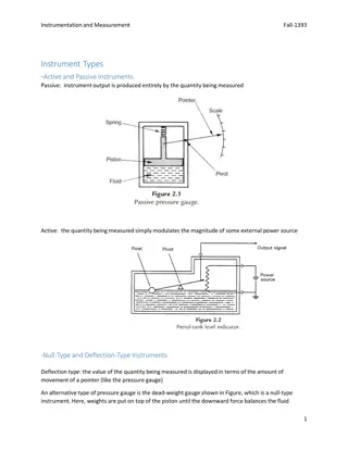
In a passive instrument, the quantity being measured is the instruments output, e.g. a pressure-measuring device. As shown in Fig 2.1, the fluid pressure is translated into a movement of a pointer against a scale. The energy expended to move the pointer is derived entirely from the change in pressure measured. There are no other energy inputs to the system. They are cheaper. e
In an active instrument, the quantity being measured modulates the magnitude of some external power source. Example is a float-type petrol tank. The change in petrol level moves a potentiometer arm, and the output signal consists of a proportion of the external voltage source applied across the two ends of the potentiometer The energy in the output signal comes from the external power source: the primary transducer float system is merely modulating the value of the voltage from this external power source.
Measured quantity is displayed in terms of the amount of movement of a pointer E.g. pressure gauge. Its accuracy depends on the linearity and calibration of the spring. It is easier to read the position of a pointer than to add and subtract weights. It is clearly more convenient to use and would normally be used in the workplace.
Pressure is measured by deducing the value of weights needed to reach this null point. E.g. deadweight gauge. Weights are put on top of the piston until the downward force balances the fluid pressure to reach the datum level. Pressure measurement is made in terms of the value of the weights needed to reach the null position. It is more accurate and its accuracy depends on the calibration of the weights. Calibration of weights is much easier than careful choice and calibration of a linear-characteristic spring. .
They vary continuously as the quantity being measured changes, e.g. the deflection-type pressure gauge . The output can have an infinite number of values within the range that the instrument is designed to measure. An analogue instrument has to be interfaced via an analogue- to-digital (A/D) converter. The addition of an A/D converter has cost implications and can degrade the speed of operation of the control system. Accuracy might be affected by the A/D converter.
Digital instruments vary in discrete steps and so has a finite number values within its range. E.g. the rev counter A cam is attached to the revolving body whose motion measured. On each revolution the cam opens and closes a switch. The switching counted by an electronic counter. A digital instrument interfaced directly microcomputer is being operations are can to be a Fig. 2.4 A Rev counter
Simply give an indication of the quantity being measured. E.g. all null-type instruments and most passive ones Can have an analogue display e.g. liquid-in-glass thermometer Can have both analogue and digital display, e.g. bathroom scale Disadvantages of Indicators Human intervention is required to read and record a measurement It is prone to error in the case of analogue output displays But digital displays are not very prone to error
They are commonly used as part of automatic control systems. They can also be found in measurement systems, where the output measurement signal is recorded in some way for later use. Measurement signal involved is an electrical voltage. It can also take other forms in some systems such as an electrical current, an optical signal or a pneumatic signal.
Smart instruments incorporate a microprocessor . Non-smart instruments do not incorporate microprocessor.
They are accuracy, precision, sensitivity, linearity etc. They are specified in the datasheet of the instruments and are considered for selection of instrument. The datasheet specifications usually apply strictly under specified standard calibration conditions. Due allowance must be made for variations in the characteristics when the instrument is used in other conditions.
This is a measure of how close the output reading of an instrument is to the correct value. The inaccuracy (measurement uncertainty) of an instrument is the extent to which its reading might be wrong. If a pressure gauge, 0 - 10 bar, has inaccuracy of 1.0% (0.1 bar), this means that a reading of 1 bar could be wrong by 10%. Taking pressure measurements with expected values between 0 and 1 bar, an instrument with a range of 0 10 bar cannot be used.
Precision describes an instruments freedom from random errors. Precision is NOT to be confused with accuracy. Repeatability is the closeness of output readings when the same input is applied repetitively over a short period of time, under the same conditions, same observer, same location and same conditions of use maintained throughout. Reproducibility is the closeness of the output readings when there are changes in the method of measurement, observer, measuring instrument, location, conditions of use and time of measurement.
Maximum error to be expected. Closely related to accuracy as some instruments have their accuracy mentioned in terms of a tolerance value. When used correctly, tolerance describes the maximum deviation of a manufactured component from some specified value. A resistor with a tolerance of 5% having a nominal value of 1000 W may have the actual value between 950 W and 1050 W.
The minimum and maximum values of a quantity that the instrument is designed to measure.
It is normally desirable that the output reading of an instrument be linearly proportional to the quantity being measured. Nonlinearity is defined as the maximum deviation from the line of best fit. It is usually expressed as a percentage the full-scale reading.
Measure of the change in instrument output that occurs when the quantity being measured changes by a giving amount. The slope of the straight line drawn on Figure 2.6. Ratio of scale deflection / value of measurand producing deflection If a pressure of 2 bar produces a deflection of 10 degrees in a pressure transducer, the sensitivity of the instrument is 5 degrees/bar. Assuming that the deflection is zero with zero pressure applied.
The following resistance values of a platinum resistance thermometer were measured at a range of temperatures. Determine the measurement sensitivity of the instrument in ohms/ C. Resistance (Ohms) Temperature ( C) Resistance (Ohms) 307 314 321 328 200 230 260 290 Solution If these values are plotted on a graph, the straight-line relationship between resistance change and temperature change is obvious. For a change in temperature of 30 C, the change in resistance is 7 Ohms. Hence the Measurement sensitivity = 7/30 = 0.233Ohms/ C.
If the input to an instrument is gradually increased from zero, the input will have to reach a certain minimum level before the change in the instrument output reading is of a large enough magnitude to be detectable. This minimum level of input is known as the threshold of the instrument. E.g., a car speedometer with typical threshold of about 15 km/h, means that, if the vehicle starts from rest and accelerates, no output reading is observed on the speedometer until the speed reaches 15 km/h. Is sometimes quoted as an absolute value. Is expressed as a percentage of the full scale reading.
There is a lower limit on the magnitude of the change in the input measured quantity that produces an observable change in the instrument output. Also sometimes specified as an absolute value or as a percentage of fsd. Major factor influencing resolution is how finely its output scale is divided into subdivisions. E.g. a car speedometer with subdivisions of typically 20 km/h. This means that when the needle is between the scale markings, we cannot estimate speed more accurately than to the nearest 5 km/h. This figure of 5 km/h thus represents the resolution of the instrument.
All calibrations and specifications of an instrument are only valid under controlled conditions of temp., pressure etc. which are defined in the instrument specification. As variations occur in the ambient temperature etc., certain static Instrument characteristics change, and the sensitivity to disturbance is a measure of the magnitude of this change. Such environmental changes affect instruments in two main ways: zero drift and sensitivity drift.
Zero drift or bias describes the effect where the zero reading of an instrument is modified by a change in ambient conditions. This causes a constant error that exists over the full range of measurement of the instrument. Zero drift or bias is a measure of how certain static characteristics of an instrument changes as the standard ambient conditions vary. Sensitivity drift or scale factor drift is the amount by which an instrument s sensitivity of measurement varies as ambient conditions change. It is quantified by sensitivity drift coefficients that define how much drift there is for a unit change in each environmental parameter that the instrument characteristics are sensitive to.
Many components within an instrument are affected by environmental fluctuations, such as temperature changes: E.g., the modulus of elasticity of a spring is temperature dependent. Figure 2.7(b) shows what effect sensitivity drift can have on the output characteristic of an instrument. Sensitivity drift is measured in units of the form (angular degree/bar)/ C. If an instrument suffers both zero drift and sensitivity drift at the same time, then the typical modification of the output characteristic is shown in Figure 2.7(c).
A spring balance is calibrated in an environment at a temperature of 20 C and has the following deflection/load characteristic. Load (Kg) Deflection (mm) 0 Load (Kg) 0 0 1 1 20 2 2 40 3 3 60 It is then used in an environment at a temperature of 30 C and the following deflection/load characteristic is measured. Load (Kg) Deflection (mm) Load (Kg) 0 0 5 1 1 27 2 2 49 3 3 71 Determine the zero drift and sensitivity drift per C change in ambient temperature.
At 20C, deflection/load characteristic is a straight line. Sensitivity = 20 mm/kg. At 30 C, deflection/load characteristic is still a straight line. Sensitivity = 22 mm/kg. Bias (zero drift) = 5mm (the no-load deflection) Sensitivity drift = 2 mm/kg Zero drift/ C = 5/10 = 0.5 mm/ C Sensitivity drift/ C = 2/10 = 0.2 (mm per kg)/ C
Figure 2.8 illustrates the output characteristic of an instrument that exhibits hysteresis. If the input measured quantity to the instrument is steadily increased from a negative value, the output reading varies in the manner shown in curve (a). If the input variable is then steadily decreased, the output varies in the manner shown in curve (b). The non-coincidence between these loading and unloading curves is known as hysteresis. Two quantities maximum input hysteresis and maximum output hysteresis, as shown in Figure 2.8.
They are normally expressed as a percentage of the full-scale input or output reading respectively. Hysteresis is most commonly found in instruments that contain springs, like passive pressure gauge and the Prony brake (used for measuring torque). Mechanical flyball rotational velocity suffer hysteresis from both of the above sources because they have friction in moving parts and also contain a spring for measuring
The range of different input values over which there is no change in output value. Any instrument that exhibits hysteresis also displays dead space, as marked on Figure 2.8. Some instruments that do not suffer from any significant hysteresis can still exhibit a dead space in their output characteristics, however.
Backlash in gears is a cause of dead space, and results in the output shown in Figure 2.9. Backlash is experienced used to convert between translational and rotational motion. characteristic commonly gearsets in
An instrument only conforms to stated static and dynamic patterns of behaviour after it has been calibrated. It can normally be assumed that a new instrument will have been calibrated when it is obtained from an instrument manufacturer. It will therefore initially behave according to the characteristics stated in the specifications. During use, however, its behaviour will gradually diverge from the stated specification for a variety of reasons:
Mechanical wear, the effects of dirt, dust, fumes and chemicals in the operating environment. The rate of divergence from standard specifications varies according to the type of instrument, the frequency of usage and the severity of the operating conditions. However, there is a time, practically, when the characteristics of the instrument will have drifted from the standard specification by an unacceptable amount. When this situation is reached, it is necessary to recalibrate, i.e readjust the instrument to the standard specifications.
1. A tungsten/5% rheniumtungsten/26% rhenium thermocouple has an output e.m.f. as shown in the following table when its hot (measuring) junction is at the temperatures shown. Determine the sensitivity of measurement for the thermocouple in mV/ C. 4.37 250 4.37 8.74 500 8.74 13.11 750 13.11 17.48 17.48 1000 mV C 2. An instrument is calibrated in an environment at a temperature of 20 C and the following output readings y are obtained for various input values y y x 13.1 13.1 5 26.2 10 26.2 39.3 15 39.3 52.4 20 52.4 65.5 25 65.5 78.6 30 78.6 Determine the measurement sensitivity, expressed as the ratio y/x.
Practise all questions at the end of Chapter 2 of the text book. Measurement and Instrumentation Principles by Alan S. Morris, Third Edition, Published by Butterworth Heineman , 2001.