Electromagnetic Surveying Methods and Applications
Electromagnetic surveying, conducted by Dr. Laurent Marescot, utilizes various methods like resistivity, induced polarization, and high-frequency techniques for exploration and investigation purposes. The electromagnetic method involves generating primary fields and detecting secondary fields to analyze ground conductivity. This method finds applications in locating mineral deposits, fossil fuels, site investigations, glaciology, and archaeology. The lecture covers equations, survey strategies, and conclusions related to electromagnetic surveying, including principles like Maxwell's equations and field measurements.
- Electromagnetic surveying
- Exploration methods
- Mineral deposits
- Field investigations
- Maxwells equations

Download Presentation

Please find below an Image/Link to download the presentation.
The content on the website is provided AS IS for your information and personal use only. It may not be sold, licensed, or shared on other websites without obtaining consent from the author. Download presentation by click this link. If you encounter any issues during the download, it is possible that the publisher has removed the file from their server.
E N D
Presentation Transcript
Electromagnetic surveying Dr. Laurent Marescot laurent@tomoquest.com 1
Introduction Electrical surveying Resistivity method Induced polarization method (IP) Self-potential (SP) method Higher frequency methods (electromagnetic surveys): Electromagnetic induction methods Ground penetrating radar (GPR) 2
Electromagnetic method Electromagnetic (EM) surveying methods make use of the response of the ground to the propagation of electromagnetic field. This response vary according to the conductivity of the ground (in S/m). Primary EM fields are generated using a alternating current in a loop wire (coil) or a natural EM source The response of the ground is the generation of a secondary EM field The resultant field is detected by the alternating currents that they induce in a receiver coil 4
Application Exploration of metalliferous mineral deposits Exploration for fossil fuels (oil, gas, coal) Engineering/construction site investigation Glaciology, permafrost Geology Archaeological investigations 5
Structure of the lecture 1. Equations in electromagnetic surveying 2. Survey strategies and interpretation 3. Conclusions 6
Maxwell equations E + B=0 Faradayinduction t H D=j Amp re Maxwell t p t D =p or j = electricalfield (V/m) E (Vs/m2) magnetic induction field B B =0 (A/m) magnetic field strenght H displacement field (C/m2) D current density charge density (A/m2) (C/m3) j p 8
B and H fields F =ev B B H = We can measure B, not H! 0 Vs permeability for vacuum Am =4 10 7 0 permeability of material B magnetic induction field Example of values for : Hematite, quartz: 1 Magnetite: 5 (Vs/m2) 9 magnetic field strenght (A/m) H
Frequencies frequency (Hz) period (s) angular velocity (rad/s) f =2 f =2 1 T T In the field, some frequencies are considered as noise and must be filtered out: Light CFF/SBB 3rd harmonic 50 Hz 16.6 Hz 150 Hz 10
Basic theory: induction EM H D=j t Amp re-Maxwell E + B=0 t Faraday 12
=+=+tan 1( L/R) 2 2 R is the resistance of the conductor L is the inductance of the conductor (or its tendancy to oppose a change in the applied field) 13
Real and imaginary components = + = +tan 1( L/ R) 2 2 S sin S cos in-phase component (real) out-of-phase component (imaginary) 14
Effect of a conductive body = + = +tan 1( L/ R) 2 2 Large conductivity (R 0 and /2): Low conductivity (R and 0): /2 15
Tilt-angle methods The receiving coil is turned until a null position is reached (no-signal): the plane of the coil then lies in the direction of the arriving field 16
Depth of penetration and skin depth depth at which the amplitude of the field reaches 1/e of its original value a the source 2 0 Skin depth: = 503 f Depth of penetration: maximum depth ze at which a conductor may still produce a recognizable EM anomaly (empirical relation) ze 100 f 17
Classification of EM methods Uniform field methods Magnetotelluric (MT) Audio-magnetotelluric (AMT) Very-Low Frequency (VLF-tilt, VLF-R) Controlled source audio-magnetotelluric (CSAMT) Dipolar field methods Twin-coil or slingram systems: dipole source is used Time-domain EM Transient EM (TEM) 19
Magnetotelluric (MT) The source are fields of natural origin (magneto-telluric fields) resulting from flows of charged particles in the ionosphere, correlated with diurnal variations in the geomagnetic field caused by solar emissions The only electrical technique capable of penetrating to the depths of interest to the oil industry (mapping salt domes and anticlines) Frequencies range from 10-5 Hz to 20 kHz 20
Telluric measurements 22 ) unit base circle area (A ) measured ellipse area (A 1 2
23 Map of A /A for a salt dome 2 1
MT measurements 2 Ex( ) 1 1 ( ) = a Z( )2 = 0 0Hy( ) 24
Audio-magnetotelluric (AMT) Use equatorial thunderstorms as sources (1 to 20 kHz). These EM fields are called sferics. Sferics propagated around the Earth between the ground and the ionosphere The very broad frequency spectrum can be filtered to select a depth of investigation up to 1 km (AMT soundings) Method sensitive to noise in urban areas 25
AMT-MT sounding 2 0.2 E H f = a 26
Very-Low Frequency (VLF-tilt) Use submarine communication waves as sources (10 to 30 kHz). The transmitters are very powerful (>1 MW).The primary EM field is planar and horizontal The depth of investigation mainly depends on the conductivity of rocks and the transmitter chosen (from 10m to 100m) Disadvantages: transmission frequently broken, difficult to find a transmitter in an appropriate direction Advantages: light, fast and easy to use 29
Very-Low Frequency (VLF-R) Gives apparent resistivity of the ground and phase shift by measuring H and E Various local radio waves can be used to chose a depth of investigation (frequency can be chosen) 32
VLF-R measurements 2 0.2 E H f = a 33
Controlled sourceAMT (CSAMT) Similar to MT but using a remote (2 to 8 km) electrical dipole as source (1 Hz to 10 kHz) The source frequency and location is known 34
Dipole-source methods Measurements tolls called twin-coil or slingram systems Tx and Rx are coils (about 1m diameter) linked by a cable which carries a reference signal in order to compensate the effect of the primary field. By this means, the system subsequently responds only to the secondary fields A decomposer spilt the secondary field into real and imaginary components (display the result as a percentage of the primary field) 36
EM31 (Geonics), 9.8 kHz, s=3.66 m EM34 (Geonics), 6.4 kHz for s=10 m 1.6 kHz for s=20 m 0.4 kHz for s=40 m EM38 (Geonics), 14.6 kHz, s=1 m 38 s: Rx-Tx distance
EM at low induction numbers (LIN) Depth of investigation depends on the distance Tx-Rx The response is proportional to ground conductivity Manufacturer adapts the Rx-Tx distance (s) and frequency ( f ) for a LIN approximation, i.e. s<< : 4 N < <1 HS B H i s2 0 a P f 503 N =s/ B is theinduction number 41
CST and VES using LIN CST: moving vertical and horizontal dipoles with various constant depth (survey principle similar to resistivity CST and tomography) VES: increasing Tx-Rx spacing around a same location point and using vertical and horizontal dipoles (survey principle similar to resistivity VES) 42
Transient EM (TEM) TEM uses a primary field which is not continuous but consists of a series of pulses separated by measurement periods when the transmitter is inactive Primary and secondary fields are clearly separated Investigation depth up to several km could be achieved, but difficult to use in shallow geophysics (no reliable information in the 0-10 m depth range) 46


")


")


")


")


")

")


, 9.8 kHz, s=3.66 m")


")


")