Understanding Vacuum: Techniques, Applications, and Classification

Explore the concept of vacuum, its applications in reducing gas concentrations and enhancing particle free paths. Learn about vacuum classification based on pressure levels and gas flow regimes. Discover the creation of vacuum using primary pumping systems and UHV technologies.

Download Presentation

Please find below an Image/Link to download the presentation.
The content on the website is provided AS IS for your information and personal use only. It may not be sold, licensed, or shared on other websites without obtaining consent from the author. Download presentation by click this link. If you encounter any issues during the download, it is possible that the publisher has removed the file from their server.
E N D
Presentation Transcript
UHV Techniques As part of the course Molecular Aspects of Catalysts and Surfaces 529-0611-00L Dr. Luca Artiglia Paul Scherrer Institut luca.artiglia@psi.ch
What is Vacuum? The term VACUUM can be used to describe these conditions: 1) Complete absence of matter (definite volume in which gases are almost absent e.g. interstellar space) 2) Physical state in which the pressure in a definite volume is smaller than in the surroundings (e.g. smaller than the atmospheric pressure) An example: gas = 2 1019 mol/cm3 (atmospheric pressure) gas = 109 mol/cm3 (orbiting satellite)
Some applications of Vacuum Reduce the concentration of a gas below a critical level (e.g. O2 in bulbs) Avoid gas-driven physico-chemical processes (e.g. experiments studying the gas-surface interaction) and increase the mean free path of particles (e.g. ion and electron spectroscopies) Thermal insulation Degasification of liquids
Vacuum classification Vacuum Pressure (torr) Number Density (m-3) M.F.P. (m) Surface Collision Freq. (m-2 s-1) Monolayer Formation Time (s) 2.7 1025 7 10 8 3 1027 3.3 10-9 Atmosphere 760 3.5 1019 4 1021 2.5 10-3 10-1-10 3 Rough 0.05 3.5 1016 4 1018 10-3-10 6 High 50 2.5 3.5 1013 50 103 4 1015 2.5 103 10-6-10 9 Very high 3.5 1010 50 106 4 1012 2.5 106 (29 days!) 10-9-10 12 Ultrahigh
Gas flow regimes The mean free path is the average distance that a gas molecule can travel before colliding with another molecule and is determined by: - Size of molecule (2r) - Pressure (p) - Temperature (T) T k . a= (2r)2p 2
The gas in a vacuum system can be in a viscous state, in a molecular state (or in a transition state) depending on the dimensionless parameter know as the Knudsen number (Kn) that is the ratio between the mean free path and the characteristic dimension of the flow channel. Molecular Flow (molecules move independently) Viscous Flow (momentum transfer between molecules) P<10-3mbar P> 1 mbar
Creation of Vacuum: pumping technology 1) Primary pumping systems: mechanical pumps that decrease the pressure from atmospheric pressure pressures close to the ultra-high vacuum (10-6-10-8 mbar) - Rough pumps (atmospheric pressure down to 10-3 mbar): membrane pumps, rotary pumps, scroll pumps, roots pumps - Turbomolecular Pumps (from the mbar to about 10-9 mbar ) 2) UHV pumping systems: pumps that work at low pressure and, thanks to their efficiency, allow reaching/improving the ultra-high vacuum (10-6-10-11 mbar). - Ion Pumps (from 10-6 mbar to 10-11 mbar) - Getter Pump - Titanium Sublimation Pump
Rough pumps: membrane and rotary pumps Membrane Rotary Combined movement of a diaphragm (plastic-rubber) and suitable valves (check, butterfly, flap valves) Consists of vanes mounted to an eccentric rotor. The vanes rotate inside a cavity Volume increased = fluid drawn into the chamber Volume decreased = fluid forced out Vanes are sealed on all edges. The rotation generates a volume expansion (gas pumping)- reduction (exhaust release) Dry pumps Can handle gas and liquids The flow rate depends on the diaphragm diameter and its stroke length Ultimate vacuum is in the mbar (larger pumps can reach 10-1 mbar) Oil pumps: oil and gas are mixed inside the pump and separated externally Multiple stage pump can generate a good vacuum (down to 10-3 mbar) Low efficiency but possibility to pump gas, gas + dust and water
Rough pumps: scroll and roots pumps Scroll Roots One of the scrolls is fixed, while the other orbits eccentrically without rotating. Compressing pockets of fluid form between the scrolls and are driven to the exhaust port Two 8-shaped synchronously counter-rotating rotors rotate contactlessly ( small gap) in a housing Dry pumps High efficiency Small gas pulsation, less vibrations Difficult maintenance Ultimate vacuum is in the 10-2 mbar range Dry pumps Can generate a good vacuum (low 10-2 mbar) No friction in the suction chamber, operation at high speed, large flow rate
Turbomolecular pumps A turbomolecular pump is used to obtain and maintain high vacuum. These pumps work on the principle that gas molecules can be given momentum in a desired direction by repeated collision with a moving solid surface. A rapidly spinning fan rotor (50000-100000 rpm) 'hits' gas molecules from the inlet of the pump towards the exhaust in order to create or maintain vacuum.
Ion pumps An ion pump is a static pump capable of reaching pressures as low as 10 11 mbar Can be turned on only at pressures around (or less than) 10-4 mbar A strong electrical voltage (typically 3 7 kV) is applied to the anode, producing free electrons. Electrons get caught by the magnetic field and rotate around it Electrons hit gas molecules ionizing them Positively charged molecules accelerates toward the cathode (grounded) at high velocity The cathode is sputtered and titanium compounds deposit on the anode The cathode acts as a getter (e.g. adsorbs inert gases)
Static pumps Non-evaporable getter Titanium sublimation Static pumps helping to establish and maintain ultra-high vacuum Static pump helping to refine the vacuum Titanium filament through which a high current (typically around 40 A) is passed periodically Porous alloys or powder mixtures of Al, Zr, Ti, V and Fe, forming stable compounds with active gases Titanium sublimates and coats the surrounding chamber walls Can be placed in narrow/difficult to reach spaces (particle accelerators) Components of the residual gas in the chamber which collide with the chamber wall react with titanium to form stable, solid products Activated by annealing to >550 K
Vacuum measurement Low vacuum: Pirani (atm. pressure 10-4 mbar) Two Pt filaments are the arms of a Wheatstone bridge and heated to a constant temperature Residual gases conduct away part of the thermal energy of the measurement filament. The amount of electrical current needed to restore its temperature is converted to a pressure readout High-Ultrahigh vacuum: hot cathode (10-4-10-11 mbar) High vacuum: cold cathode (10-4-10-9 mbar) 3 electrodes: filament, collector, grid 2 electrodes: anode, cathode + permanent magnetic field (works like a ion pump!) The pressure is measured through a gas discharge in the gauge head. The gas discharge is obtained by applying a high voltage The filament emits electrons, which are attracted to a polarized grid Residual gas molecules are ionized by the electrons and attracted by the collector. Pressure reading is determined by the electronics from the collector current.
TPD Temperature Programmed Desorption
Temperature programmed desorption* Ultra high vacuum can be used to study the adsorption/reaction of molecules on a surface (monolayer formation time in UHV 103-106 s). Discussion based on Langmuir ad-(de-)sorption isotherm Kinetics Langmuir Adsorption-Desorption d = n des r k = Adsorption is localized (adsorbed particles are immobile) n dt If k (rate constant) is described by an Arrhenius eq.: Substrate surface is saturated at = 1 ML (all adsorption sites occupied) E des = k nexp n RT No interactions between the adsorbed particles The rate law is then referred to as the Polanyi-Wigner equation: E d n des = = r exp n des dt RT n: n: : Edes: Pre-exponential factor Desorption order Surface coverage Activation energy for desorption *Resource for furtherreading: Temperature-Programmed Desorption (TPD). Thermal Desorption Spectroscopy (TDS), Sven L.M. Schroeder and Michael Gottfried, June 2002, available online.
Temperature programmed desorption A typical TPD experiment (UHV): Clean sample surface exposed to a precise amount of gas (usually measured in Langmuirs 1 L = 10 6 Torr s) Sample placed in front of a quadrupole mass spectrometer (QMS) and heated with a precise rate ( ) The quadrupole acts as a filter, separating ions with different m/z, which are then collected A typical spectrum shows the intensity of a specific m/z vs. temperature
Temperature programmed desorption If the pumping rate is faster than the desorption rate (no readsorption) a series of separated peaks can be recorded (each of them corresponding to a surface desorption process) Tm ~?( ???? ??) ~ n Pressure drop gives information about the order of the desorption process Initial increase is mainly determined by Edes A TPD experiment can give important information: Heat of desorption Surface coverage (quantification of the monolayer) Surface reactivity (gas-substrate interaction, adsorption sites) Kinetics of desorption
Temperature programmed desorption Spectral interpretation is most commonly performed using the Polanyi-Wigner equation In a TPD experiment is the heating rate, defined as = dT/dt = const. Thus dt = dT/ can be substituted in the equation to give E 1 d n des = exp n dT RT When T = Tmax 2 E d d d d dr 1 n n des = = + = = 0 n = ; rdes ; 0 des 2 2 m dt dT dT dT dT RT = =m T T T T m n E E 1 n n n des des + = exp ; 0 n 2 m RT RT 1 n n E E n n des n des = exp ; 2 m RT RT m 1 n E E n des n des This equation can be used to obtain Edes from TPD spectra (see the next slides) = exp ; 2 m RT RT m
First order kinetics (molecular) A A ( ) ( ) ads g E E E dt d des des des = = exp ; exp ; n 2 m RT RT RT m Spectra obtained at different The desorption peak areas depend on The desorption peaks are asymmetric Tm constant with increasing Tm increases with Edes
First order kinetics: approximate evaluation of Edes In 1962 Redhead, assuming that activation parameters are independent of surface coverage and that desorption followed 1st order kinetics, derived a simple equation.* E E des des = exp ; Solving this equation for Edes gives: 2 m RT RT m E The second part in the brackets is small relative to the first, and can be approximated to 3.64 (error is less than 1.5% for 108 < / < 1013 K-1) T m des = ln ln E RT m des RT m Tm and are determined experimentally . The activation energy from a single desorption spectrum can be estimated using an approximate value for . = 1013 s-1 is a commonly chosen value. As an example: in this case Tm= 117 K. Tm Assuming =1.0 1013 s-1 and =2 K/s Edes= 29.5 kJ/mol *P. A. Redhead, Vacuum 12, 203-211 (1962).
First order kinetics: approximate evaluation of Edes from curves having different A series of spectra for the same is acquired employing different = dT/dt = const. From each spectrum, the temperature of the desorption rate maximum Tm is determined 2 E E E E T des des m des des = exp ; Taking the ln and rearranging.. = + ln ln 2 m RT T R R RT m m Plotting of ln(T2m/ ) vs. 1/Tm for a series of values provides Edes from the slope and from the intercept with the ordinate .
Second order kinetics (recombinative desoprtion) + A B AB AB (g ) ads ads ads E E E 2 dt d des n des 2 = des exp ; = exp ; n 2 m RT RT RT m Spectra obtained at different Tm shifts with increasing Characteristic nearly symmetric peak shape with respect to Tm . (Tm) is a half of the value before desorption 2 E E T m des des = + ln ln dividing by the units and rearranging we obtain: R T R m Plotting the ln(T2m/ ) vs. 1/Tm for a series of values provides Edes from the slope and (if is known) from the intercept with the ordinate
Leading edge analysis But the activation parameters often depend on the coverage and temperature! Increasing , Tm shifts negatively due adsorbate-adsorbate interactions Leading edge . Habenschaden and K ppers leading edge method* Leading edge: almost unchanged The rate of desorption is evaluated from each single leading edge E n E n des des = r exp = + + ln(r ) ln( ) ln n des n des RT RT ln(rdes) plotted vs. 1/T. The slope gives Edes and the intercept with y gives *E. Habenschaden, J. K ppers, Surf. Sci. 138, L147 (1984).
An example of TPD applied to the study of a catalytic reaction
CO and O2 desorption Procedure: 50 L of gas dosed on the clean foil at RT. Sample heated from RT to 700 C with =10 K/s Molecular adsorption (first order) Two main desorption peaks (a foil is polycristalline) at ca. 110 and 225 C Dissociative adsorption (recombinative desorption process) Multiple desorption peaks at higher temperature than for CO (larger Edes)
Temperature programmed reaction (TPR) Procedure: 50 L of CO dosed on the clean foil at RT. Sample heated from RT to 700 C with =10 K/s while flowing 3 10-7 Torr of O2. Sample surface saturated with CO CO desorption peaks intensity decreases As the CO starts to desorb, the partial pressure of O2 decreases and the signal of CO2 increases Procedure: 50 L of O2 dosed on the clean foil at RT. Sample heated from RT to 700 C with =10 K/s while flowing 3 10-8 Torr of CO. Sample surface saturated with O2 CO2 is produced immediately, but its signal goes down above 300 C CO2 production correlated with CO desorption
In case of E-R mechanism the reaction should start immediately after introducing one of the reagents (in the presence of the other adsorbed) In both TPR experiment CO2 production correlates with the presence of both reagents on the sample surface TPR performed after CO pre-adsorption clearly demonstrates competition between the reagents for the adsorption sites (especially reaction at high temperature). CO is blocking the adsorption sites (poisoning effect), and some energy (temperature) is required to remove part of it and allow oxygen to adsorb and split TPR performed after O2 pre-adsorption clearly demonstrates that adsorbed CO is necessary for CO2 formation (no more CO2 formed above 300 C These model experiments support the hypothesis that a L-H mechanism operates, in good agreement with the literature
XPS X-ray Photoelectron Spectroscopy Resource for further reading: Surface Analysis by Auger and X-ray Photoelectron Spectroscopy, D. Briggs, J.T. Grant, eds., IM Publications and SurfaceSpectra Ltd., 2003 Photoelectron Spectroscopy, Principles and Applications, S. H fner, eds. Springer-Verlag Berlin Heidelberg 1995,1996,2003.
What is XPS? Nobel prize (physics) 1981 Nobel prize (physics) 1921 Photoelectric Effect Albert Einstein Binding energy! The binding energies are characteristic of specific electron orbitals in specific atoms XPS lines are identified by the shell from which the electron is emitted Photoelectrons can escape only a few nm (this depends on their KE) Surface sensitive!
XPS in a nut-shell X-ray photoelectron spectroscopy (XPS) is a classical method for the semiquantitative analysis of surface composition It is also referred to as Electron Spectroscopy for Chemical Analysis (ESCA) It is based on the photoelectric effect, i.e., emission of electron following excitation of core level electrons by photons It is surface sensitive because of the low inelastic mean free path of electrons An XPS setup consists of a X-ray source, a sample chamber and an electron analyzer XPS requires a source of X-rays, i.e., either from a lab-based anode or from a synchrotron Traditionally, XPS works only in ultrahigh vacuum because of scattering of electrons in gases XPS can also be performed in the mbar pressure range 31
Electron energy analyzer The most often used type of electron kinetic energy analyzers is composed of an electrostatic lens and a hemispherical analyzer Electrostatic lens decelerates electrons to a fixed (pass) energy in the range of a few to 100 eV and at the same time focusses them on an entrance slit of the hemispheric analyzer Electrons travel between two concentric hemispheres with a constant potential difference and reach a detector with one dimension aligning a small kinetic energy range A spectrum is obtained by sweeping the lens electric field to cover specific kinetic energy ranges of the photoelectrons Operation of an electron analyzer requires high vacuum to avoid scattering losses of electrons and to protect the detector 33
The photoemission process Photoelectron Kinetic energy EV EF Valence band Binding energy Core hole Photon Core levels KE = h BE for a solid KE = h IP for a gas : photoelectric workfunction 34
Fate of core hole Auger electron emission or X-ray fluorescence Photoemission Relaxation 35
Why is XPS surface sensitive? XPS probe depth Ekin= h -BE- X-ray photons can penetrate m but X-ray Ekin= h -BE- - Only photoelectrons from the first layers can escape without energy loss e Inelastic mean free path ( ) and probing depth strongly depends on the kinetic (and thus photon) energy d Depth profiles can be obtained either by varying the incident photon energy (tunable x-ray source) or by varying the detection angle ( ) Contribution of atom in depth d to PE peak: Contribution to the photoelectron signal from atoms below the surface decreases exponentially In normal emission 95% of the signal comes from a 3 depth 36
Inelastic background Ekin= h -BE- Photoelectrons from deeper layers lose part of their energy (inelastic collisions) and are emitted with reduced KE (> BE) X-ray Ekin= h -BE- - e XPS spectra show characteristic "stepped" background (intensity of background towards higher BE of photoemission peak is always larger than towards lower BE) d 2s 2p 3s 3d 1000 Binding energy (eV) 0 Kinetic energy (eV) 1000 0 38
A photoelectron spectrum in more detail O 1s Ti 2p3/2 Photoemission Intensity (arb. units) TiO2Survey hv=730 eV Peak shape Spin-orbit splitting Ti 2p1/2 Auger peaks Ti 2s Ti LMM Ti L2,3M2,3V Auger peaks Shake-up C 1s O KLL Ti 3p O 2s Background shape Ti 3s VB 600 500 400 300 200 100 0 Binding Energy (eV) Binding energy scale (eV) 39
Spin-orbit splitting n: principal quantum number l: orbital angular momentum quantum number s: spin angular momentum quantum number j =|l s|: total angular momentum quantum number l = 0 .. s 1 .. p 2 .. d 3 .. f For l = 0, s levels are singlets, no splitting For l > 0, p,d,f levels give rise to doublets. The spin angular momentum of electrons left in an orbital couple with the angular momentum vector n 2p3/2 The degeneracy 2j + 1 determines the possibility for parallel and anti-parallel pairing The ratio between the degeneracies (R), (2j++1)/(2j-+1), determines the relative peak ratio of the two peak components. j = l - s j = l + s E between two components = spin orbit splitting. Magnitude of spin-orbit splitting increases with Z and decreases with distance from nucleus (same energy level, E increases with decreasing l) 40
Core level chemical shifts Position of orbitals in atom is sensitive to its chemical environment Chemical shift correlated with overall charge on atom (more positive charge = increased BE) number of substituents substituent electronegativity formal oxidation state (depending upon ionicity/covalency of bonding) Citric acid Chemical shift analysis is powerful tool for chemical composition, functional group and oxidation state analysis 41
Secondary structure of a spectrum Interaction of the photoemitted electron (along its trajectory) and the remaining electrons: final state effects (satellite peaks) Shake-up. An electron of the VB can be excited. The energy of this excitation will be deducted from the kinetic energy of the photoelectron. Relevant in metals, in which the valence and conduction bands overlap, empty states are available at very low excitation energies Simultaneous excitation of a specific wave mode in the sample (e.g. surface plasmons). The kinetic energy loss is h s ( s is the plasmon frequence), and will repeat at multiples of s 42
Secondary structure of a spectrum Cr 2p3/2 Multiplet splitting. Arises when an atom contains unpaired electrons (e.g. Cr3+, 3p63d3). During the photoemission process, there can be coupling between the unpaired electron in the core with the unpaired electrons in the outer shell. This can create a number of final states, which will be seen in the photoelectron spectrum as a multi-peak envelope. This creates different final states, depending on the orientation of the spin of the unpaired electrons 43
Estimate of the signal intensity Contribution of element A at depth d to photoemission signal d ( ) d ( ) ( ) = cos I c h e Analyzer A T A i , j Analyzer A X Analyzer transmission Concentration of element A at depth d Angular acceptance Attenuation from depth d at detection angle Photon flux Subshell ionization cross section Cross section - (KE) - is the probability to have the photoemission event 1015atoms cm-2(equivalent to a monolayer) lead to about 10-3photoelectrons per incident photon Typical photon flux: 1012s-1, leads to about 109photoelectrons s-1 44
Ambient pressure x-ray photoelectron spectroscopy But XPS is historically bound to high ultra-high vacuum Pressure gap Material gap APXPS has partially filled the gaps!* XPS up to 5 mbar (soft x- rays) and 50 mbar (tender x-rays) Possibility to investigate real samples (powders, semiconductors) Page 45 *O. Karsl o lu, H. Bluhm, in Operando Research in Heterogeneous Catalysis, Vol. 114, Springer Series in Chemical Physics pp 31- 57.
Depth profile If a tunable X-ray source (from a synchrotron) is available, a given electronic level can be excited with varying photon energies, resulting in varying photoelectron kinetic energies. Since the IMFP monotonously increases with increasing kinetic energy above about 100 eV, XPS can be used to obtain depth profiles of elements or their chemical state. Au0 Oxidation of Au exposing a gold foil (T=373 K) to 0.3 mbar O3 (1%) in O2 Au + New component in the Au 4f spectrum, associated with cationic gold The appearance of a O 1s peak confirms that a Au-O bond forms Au + intensity is maximum at h =175 eV, and decreases with increasing excitation energy (surface cationic gold)
Depth profile The Au +/Au0 ratio can be plotted vs. kinetic energy ( IMFP) It decreases demonstrating that the oxide stays at the surface The experimental data can be fitted with a function reproducing the attenuation of the photoemission signal either in a uniform oxide layer (thickness t straight line) or in patches of oxide overlayer (dashed line) supported on a semi-infinite metallic support t=0.3 nm suggests that a O-Au-O trilayer forms at the surface
The solid-gas interface @ NAPP (SLS-PSI) Static chamber @ NAPP* Flow tube configuration Heated sample holder. Sample powder pressed, dispersed in ethanol and drop-casted on a gold foil Fast heating (e.g. from RT to stable 300 C in a few seconds) Page 48 *F. Orlando, et al. Top. Catal. 2016, 59, 591.
Carbon monoxide oxidation on Pt/CeO2 Metal NPs (Pt, Pd, Au) supported on reducible oxides showed the best performance in the low temperature oxidation of carbon monoxide* For CeO2: adsorption and activation of oxygen preferentially occur on the support, whereas carbon monoxide is adsorbed and supplied by the metal# Under catalytically relevant conditions: rapid reoxidation of ceria. Ce3+ generated in the catalytic cycle is difficult too short lived to be detected under steady state conditions. Studies employing time-resolved techniques are required to gather more information about the evolution of the active sites and their role in the reaction mechanism Page 49 * I. X. Green, et al., Science 2011, 333, 736. M. Cargnello, et al., Science 2013, 341, 771. J. Saavedra, et al., Science 2014, 345, 1599. # R. Kopelent, et al., Angew. Chem. Int. Ed. 2015, 54, 8728. Page 49
Carbon monoxide oxidation on Pt/CeO2 Time-resolved RXES of Pt(1.5%)/CeO2 (ca. 1.2 nm diameter Pt NPs on powdered ceria) oxygen excess (1%CO, 4% O2)*. Pulsed experiment: from CO+O2 to CO+inert The Ce3+ concentration increases, thus oxygen from ceria participates in the oxidation of carbon monoxide. The initial rate of ceria oxidation is >10 times higher than that of reduction. Active Ce3+ is short lived Presence of spectator Ce3+ (not involved in the catalytic process) probably formed during pretreatment of catalyst. OPEN ISSUES What is the effect of the activation in hydrogen? Are the active sites located at the metal/oxide interface? Exploit the surface sensitivity of XPS. Page 50 * R. Kopelent, et al., Angew. Chem. Int. Ed. 2015, 54, 8728.


")


")


")


")