Matrix Functions and Taylor Series in Mathematics

A detailed exploration of functions of matrices, including exponential of a matrix, eigenvector sets, eigenvalues, Jordan-Canonical form, and applications of Taylor series to compute matrix functions like cosine. The content provides a deep dive into spectral mapping, eigenvalues, eigenvectors, and their implications in matrix operations.

• Mathematics
• Matrix Functions
• Taylor Series
• Spectral Mapping

tor_ows Follow

Uploaded on Oct 03, 2024 | 0 Views

Download Presentation

Please find below an Image/Link to download the presentation.

The content on the website is provided AS IS for your information and personal use only. It may not be sold, licensed, or shared on other websites without obtaining consent from the author. Download presentation by click this link. If you encounter any issues during the download, it is possible that the publisher has removed the file from their server.

Presentation Transcript

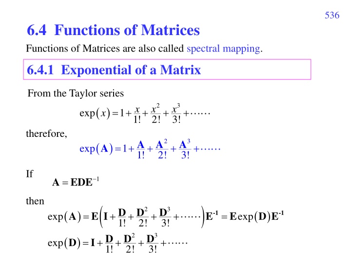
1. 536 6.4 Functions of Matrices Functions of Matrices are also called spectral mapping. 6.4.1 Exponential of a Matrix From the Taylor series 2 3 x x x ( ) x = + + + + exp 1 1! 2! 3! therefore, 2 3 A A A ( ) A = + + + + exp 1 1! 2! 3! If = 1 A EDE then ( ) 2 3 D D D ( ) A ( ) D E -1 -1 = + + + + = E I E E exp exp 1! 2! 3! 2 3 D D D ( ) D = + I + + + exp 1! 2! 3!

2. 537 (Case 1): If A has a complete eigenvector set, then 0 0 0 2 1 2! 1 0 2 = D + 0 0 N + + ( ) D 1 0 0 = exp 1 2 2 + + + 0 1 0 2 3 D D D + + + + = I 2! 2 1! 2! 3! 2 N + + + 0 0 1 2! N exp( ) 0 0 0 0 1 exp( ) 2 = 0 0 exp( ) N

3. 538 (Case 2): If A does not have a complete eigenvector set, then 1 0 1 0 0 D 0 0 0 0 k 1 0 D k 2 = D I or = k = D D k k 0 0 0 0 1 0 0 D k K 0 k S 0 0 0 0 1 S 2 3 D D D 2 + + + + = I 1! 2! 3! 0 0 S K 2 k 3 k D D D ( ) = = + I + + + where S D k exp k k 1! 2! 3!

4. 539 1 0 1 0 0 k 0 k 2 k 3 k D D D = + I + + + S k = D If k 1! 2! 3! k 0 0 0 0 1 k 0 k then m n = S , 0 if m > n, k 2 k 3 k ( ) = + + + + = S , 1 exp n n k k 1! 2! 3! k 1 n m + = S , m n k ! k n m n m = 1 n 1 1 1 n m + = = + ( )!( )! ( )! ! m n m n m k k n m = = 0 1 ( ) = exp ( )! n m k

5. 540 Therefore, 1 1! 1 2! 1 1! 1 e e e e k k k k ( 1)! M 0 e e k k ( ) = = D S exp 1 2! 1 1! e e k k k 0 0 e e k k 0 0 0 k

6. 541 [Example 1] If 2 1 0 2 2 2 0 = A 1 2 ( ) exp A determine (Solution): The eigenvalues of A are 2, 2, 2. The Jordan-Canonical form of A is 2 0 0 1 2 0 0 1 2 = 1 A EDE = D 1 0 1/ 2 1 0 1/ 2 0 0 0 0 2 0 2 0 1 0 = = 1 E E , 0 2

7. 542 ( ) A ( ) D E = 1 E exp exp 2 2 2 / 2 e e e e ( ) D where = 2 2 exp 0 0 e e 2 0 Therefore, 2 2 2 2 e e 2 e e e e e ( ) A = 2 2 2 exp 2 2 2 0 e

8. 543 6.4.2 Functions Using Taylor Series ( subsection ) (1) cos(A) ( ) cos A To derive 2 4 6 x x x x = + + cos 1 we can apply 2! 4! 6! 2 4 6 A A A ( ) A = I + + cos 2! 4! 6! D ( ) 2 4 6 D D ( ) D E = + + = E ) 1 1 E I E cos 2! 4! 6! ( ) ( 2 4 6 D D D = + + D I cos where 2! 4! 6! = if 1 A EDE

9. 544 (Case 1) When A has a complete eigenvector set, then 0 0 = 2 1 1 2! 4! + = ( ) ( 0 cos cos = 0 0 1 2 D 2 1 0 0 N + 0 0 2 2 2 2 + 0 1 0 2 4 D D I 2! 4! 2! 4! 2 N 2 N + 0 0 1 2! 4! cos 0 0 0 1 ) ( ) D 2 ( ) 0 0 cos N

10. 545 (Case 2) When A does not have a complete eigenvector set, then 1 0 1 0 0 k D 0 0 0 0 1 0 k D 2 = = D D k 0 0 0 0 1 k 0 0 D K 0 k S 0 0 0 0 1 S 2 4 6 D D D 2 + + = I 2! 4! 6! 0 0 S K 2 k 4 k 6 k D D D ( ) = = I + + where S D cos k k 2! 4! 6!

11. 546 if m > n, m n = S , 0 k 2 k 4 k 6 k ( ) = + + = S , 1 cos n n k 2! 4! 6! k (1) If n m is positive and even, 2 ( 1) (2 )! n m + = 2 k S , m n k n m = n m ( )/2 ( 1) m n m + = 2 k + n m (2 )!( )! n = n m ( 1) (2 )!( ( )/2 + n m ( )/2 n m = = 2 k 2 )! n m = 0 n m ( )/2 ( 1) ( n m ( ) = cos )! k

12. 547 (2) If n m is positive and odd, 2 ( 1) (2 )! n m + = 2 k S , m n k n m = n m + ( 1)/2 ( 1) m n m + n m + = 2 k 1 = + n m (2 )!( )! n 2 = n m + ( 1)/2 + n m + n m + ( 1)/2 ( 1)/2 ( 1) (2 ( 1) ( ( ) + = = 2 k 1 sin + 1)!( )! )! n m n m k = 0 1 1 cos sin cos 1! cos 2! k k k 1 0 sin 1! k k ( ) = = D S 1 cos cos k k 2! k 1 0 0 cos sin 1! cos k k 0 0 0 k

13. 548 (2) sin(A) 3 5 x x x x = + sin 1! 3! 5! (Case 1) When A has a complete eigenvector set and 0 0 0 1 0 = 1 A EDE 2 = D 0 0 N then sin 0 0 0 1 0 sin ( ) D 2 ( ) A = = S sin = 1 ESE sin 0 0 sin N

14. 549 (Case 2) When A does not have a complete eigenvector set and = 1 A EDE 1 0 1 0 0 k D 0 0 0 0 1 0 k D 2 = = D D k 0 0 0 0 1 k 0 0 D K 0 k then S 0 0 0 0 1 S ( ) A 2 = = 1 S ESE sin 0 0 S K

15. 550 S 0 0 0 0 1 S ( ) A = 1 ESE sin 2 = S 0 0 S K m n = S , 0 if m > n, k ( ) = S , sin n n k k n m ( 1)/2 ( 1) ( ( ) = S , cos m n if n m is positive and odd, k )! n m k n m ( )/2 ( 1) ( n m ( ) = S , sin m n if n m is positive and even k )! k

16. 551 (3) In general, ( ) 0 1! ( ) 0 2! ( ) 0 3! if f f f ( ) f x ( ) 0 = + + + + 2 3 f x x x and = 1 A EDE then ( ) A ( ) D E = 1 E f f ( ) 0 1! ( ) 0 2! ( ) 0 3! f f f ( ) D ( ) 0 = + + + + 2 3 where D D D f f

17. ( ) A ( ) D E 552 = 1 E f f ( ) 0 1! ( ) 0 2! ( ) 0 3! f f f ( ) D ( ) 0 = + + + + 2 3 where D D D f f (i) When A has a complete eigenvector set and 0 0 = ( ) 1 0 f = 0 0 1 2 D 0 0 N 0 0 0 f then ( ) f ( ) D 2 ( ) 0 0 f N (ii) However, the form of f(D) is rather complicated if A does not have a complete eigenvector set.

18. 553 6.5 Generalized Norm For a vector = x [1] x [2] x [ 1] [ ] x N x N 1 N = (1) Norm (L norm): x = [ ] x n 0 n (2) L2 norm (conventional norm): 1 N = 2 x = [ ] x n 2 0 n (Physical meaning: Distance)

19. 554 1 N = x = [ ] x n 0 n 1 N = x = [ ] x n (3) L1 norm: 1 0 n (Physical meaning: Sum of Amplitudes) [Example 1] 2 2 12,5 = 12 +5 =13 2 [12,5] 5 1 12,5 =12+5=17 13 12

20. 555 1 N = x = [ ] x n 0 n x =Max [ ] x n (3) L norm: (Physical meaning: The maximal amplitude) 1 N ( ) lim [ ] x n [ ] Max x n Note: = 0 n 1 N lim [ ] x n [ ] Max x n = 0 n If there are M entries of |x[n]| that equals to Max|x[n]| 1 N ( ) lim [ ] x n [ ] M Max x n = N 0 n 1 = 1/ lim [ ] x n [ ] [ ] M Max x n Max x n = 0 n

21. 556 1 N = x = [ ] x n 0 n lim (L norm) (Also call as the L0norm) ( 0 (5) 0 1 N = ) x lim =lim [ ] x n Note that 0 0 n ( ) x lim =K 0 where K is the number of points such that x[n] 0 (Physical meaning: The number of nonzero points) The L2 norm is easier for optimization, but it often happens that using the L0or the L1norm can obtain even better optimization results.

22. 557 [Norms of a Matrix: Definition 1] 1 1 M N A = [ , ] A m n = = 0 0 m n 1 1 M N L2 norm: (also call the Frobenius norm): 2 A = [ , ] A m n 2 = 1 = 1 0 N 0 m n M A = [ , ] A m n L1 norm: 1 = = 0 0 m n L norm: (also call the max norm): A = [ , ] Max A m n , m n ( ) A lim =K L0 norm: 0 where K is the number of points that satisfy A[m, n] 0

23. 558 [Example 2] 1 2 3 1 = A 2 0 1 2 1 L2 norm: 4(1 ) 3(2 ) 3 + + = 2 2 2 5 4 1 3 2 3 13 + + = L1 norm: 3 L norm: 8 L0 norm:

24. 559 [Norms of a Matrix: Definition 2] Note: In fact, a more standard definition for the norm of a matrix is: Ax A x = sup x 0 where sup (supremum) means the least upper bound. The norm with this definition is called the operator norm. One possible application of the operator norm passivity of electrical components. is to determine the For image processing and machine learning applications, it is more often to use the same definition of the norms of a vector to define the norms of a matrix, as on page 553. The norms on page 553 are also called "Entry-wise" matrix norms or vector-based norms.

25. 560 6.6 Markov Model 6.6.1 Definitions State Vector: ( ) t ( ) ( ) ( ) t T = x , , , x t x t x 1 2 N In a Markov model, (1) x1(t), x2(t), , xN(t) can be expressed as linear combinations of {x1(t 1], x2(t 1], , xN(t 1]} ( ) ( ) ( ,1 1 ,2 2 1 m m m x t a x t a x t = + ) ( ) + + 1 1 a x t , m = 1, 2, , N: m N N (2) 0 1 a , m n N = 1 a (3) for n = 1, 2, , N: , m n = 1 m

26. 561 N = Note that, if 1 a , m n = 1 m then N N ( ) ( ) t ( ) ( ) ( ) = + + + 1 1 1 x a x t a ,2 2 x t a x t ,1 1 , m m m m N N = = 1 1 m m N N N ( ) ( ) ( ) = + + + 1 1 1 a x t a ,2 2 x t a x t ,1 1 , m m m N N = = = 1 1 1 m m m N N ( ) t ( ) = 1 x x t m m = = 1 1 m m Many problems in physics, environment, and social science can be expressed by the Markov model.

27. 562 Markov Model (Matrix Form) ( ) t ( ) 1 = x Ax t a a a a a a a a 1,1 1,2 1, 1 1, N N 2,1 2,2 2, 1 2, N N = A a a a a 1,1 1,2 1, 1 1, N N N N N N a a a a ,1 ,2 , 1 , N N N N N N ( ( ) ) ( ) ( ) 1 1 x t x t x t x t 1 1 2 2 ( ) ( ) t = = x 1 t x ( t ) ( ) ( ) t 1 x t x t 1 N x 1 N x ( ) 1 N N

28. 563 [Example 1] Migration Model Suppose that, every year, (1) 10% of the people lived in the city move to the suburb and 5% of the people lived in the city move to the countryside every year (2) In the suburb, 5% of the people move to the city and 5% of the people move to the countryside every year. (3) 10% of the people lived in the countryside move to the city and 10% of the people lived in the countryside move to the suburb.

29. 564 ( ) t ( ) 1 = where X AX t ( ) ( ) ( ) city suburb countryside x t x t x t 0.85 0.1 0.05 0.05 0.9 0.05 0.1 0.1 0.8 1 ( ) t = = X A 2 3 ( ) ( ) ( ) 0.85 0.1 0.05 0.05 0.9 0.05 0.1 0.1 0.8 ( ( ( 1) 1) 1) x t x t x t x t x t x t 1 1 = 2 2 3 3

30. 565 [Example 2] Water Cycle System Suppose that, every year, (1) 20% of the water in the air will precipitate to the land through rain or snow, 60% of the water in the air will precipitate to the sea. (2) 10% of the water in the land will flow into the sea and 5% of the water will evaporate into the air. (3) Also, 1% of the water in the see will evaporate to the air every year.

31. 566 ( ) t ( ) 1 = where X AX t ( ) ( ) ( ) 0.2 0.2 0.6 0.05 0.85 0.1 0.01 0 0.99 air land sea x t x t x t 1 ( ) t = A = X 2 3

32. 567 6.6.2 Analysis In Example 1, suppose that, initially, the populations of the city, the suburb, and the country are 50,000, 50,000, and 100,000. (1) Determine the populations of the three places 1 year, 2 years, and 10 years later. (2) Also, determine what will the populations of the three places converge to. 0.85 0.05 0.1 0.1 0.9 0.1 0.05 0.05 0.8 = A Eigenvector-eigenvalue decomposition -1 = where A EDE 3 5 2 0.1 0.5 0.2 0.1 0.5 0.2 0.1 0.5 0.8 1 1 0 1 0 0 0 0 0 = 1 = = E E D 1 0.8 0 0 1 0.75

33. 568 50000 50000 100000 ( ) 0 = X Initial 55000 60000 85000 ( ) 1 ( ) 0 = = After one year X AX 58250 68000 73750 ( ) 2 ( ) 1 = = X AX After two years 61990 94631 43379 After ten years ( ) 10 ( ) 0 ( ) 0 10 -1 = = = 10 X A X ED E X 1 0 0 0 0 0 = 10 10 D (0.8) 10 0 (0.75)

34. 569 To determine what will the populations of the three places converge to, we can apply ( ) ( ) lim lim 0 lim t t ( ) 0 -1 = = t t X A X ED E X t t Since t 1 0 0 0 0 0 1 0 0 0 0 0 0 0 0 = = t t D lim t (0.8) 0 t (0.75) 3 5 2 1 1 0 1 0 0 0 0 0 0 0 0 0.1 0.5 0.2 0.1 0.5 0.2 0.1 0.5 0.8 100000 50000 50000 ( ) t = X lim t 1 0 1 60000 100000 40000 ( ) t = X lim t

35. 570 In Example 2, suppose that, initially, the amounts water in the air, in the land, and in the sea are x1(0), x2(0), and x3(0), respectively. (1) Determine the amounts of water in the air, the land, and the sea after 10 years. (2) Also determine what will the amounts of the water in the three places converge to. 0.2 0.05 0.01 0.2 0.85 0.6 0.1 0.99 Eigenvector-eigenvalue decomposition 3 1 3.3595 4 16.7977 1 220 17.9799 2.3595 1/ 227 1/ 227 1/ 227 0.01615 0.05723 0.00126 0.28892 0.02097 0.00356 = A 0 -1 = A EDE 1 0 0 0 0 0 = E = D 0.8619 0 0.1781 -1 = E

36. 571 After ten years 1 0 0 0 0 0 ( ) 10 ( ) 0 ( ) 0 ( ) 0 10 10 -1 -1 = = = X A X ED E X E E X 0.2263 0 3.2098 10 8 1 0 0 0 0 0 10 (0.8619) 10 0 (0.1781) ( ) ( ) ( ) 10 ( ) ( ) ( ) 0 ( ) ( ) ( ) 0 ( ) ( ) ( ) 0 + + + + + + 10 10 0.01687 0.07900 0.90413 0 0 0.02617 0.23515 0.73869 0 0 0.01293 0.01283 0.97424 0 0 x x x x x x x x x x x x 1 1 2 3 = 2 1 2 3 3 1 2 3

37. 572 To determine what will the amounts of the water in the three places converge to, ( ) ( ) lim lim 0 t t Since 1 0 lim 0 (0.8619) 0 0 1 0 0 lim 0 0 0 0 0 0 ( ) ( ( ) ( ( 1 0 227 ( ) 0 -1 = = t t X A X ED E X lim t t t 0 0 1 0 0 0 0 0 0 0 0 = = t t D t t (0.1781) ( ) t ( ) 0 -1 = X E E X t ) ) ) 3 ( ) 0 ( ) 0 + + 0 x x x ( ) ( ) ( ) 227 4 227 220 1 2 3 = x t x t x t 1 ( ) 0 ( ) 0 + + lim t 0 x x x 2 1 2 3 ( ) ( ) 0 ( ) 0 3 + + x x x 2 3

38. 573 [Theorem 1] For a Markov model matrix, (i) At least one of the eigenvalue is = 1. (ii) Other eigenvalues are no larger than 1. (iii) Moreover, if the multiplicity of = 1 is 1, then the eigenvector corresponding to = 1 determines the ratio of x1(t) : x2(t) : : xN(t) in the convergence case (t ). (Proof): Suppose that A is the transfer matrix of a Markov model. (i) To show 1 must be an eigenvalue of A: = 1 A LAL If 1 1 0 1 = -1 where 1 0 1 1 1 1 0 1 0 1 0 0 -1 = L L 0 0 0 0 1 0 0 1 0 0 0 0 1 0 0 1

39. 574 1 1 1 1 a a a a 2,1 2,2 2, 1 2, N N = LA a a a a 1,1 1,2 1, 1 1, N N N N N N a a a a ,1 ,2 , 1 , N N N N N N 1 0 0 0 a a a a a a a 2,1 2,2 2,1 2, 1 2,1 2, 2,1 N N = = 1 A LAL 1 a a a a a a a a a a 1,1 1,2 1,1 1,1 1,1 1, 1 1, N N a N N a N N N a N N a ,1 ,2 ,1 , 1 ,1 , ,1 N N N N N N N N N a a a a a a 2,2 2,1 2, 1 2,1 2, 2,1 N N ( ) ( = ) A I det 1 det 1 a a a a a a a a 1,2 1,1 1,1 1, a 1 1, 1,1 N a N N N N N N N a a ,2 ,1 , 1 ,1 , ,1 N N N N N N N N

40. 575 ( ) = = A I det 0 1 for Therefore, 1 = 1 should be one of the eigenvalues of A1and hence A (note that A and A1are similar) . (ii) To show 1 is the largest eigenvalue of A: If 2= A A T then A2and A have the same eigenvalues since det(A I) = det(A2 I). If g = [g1, g2, , gN]Tis an eigenvector of A2and the corresponding eigenvalue is . Without the loss of generalization, we suppose that |gp| |gn| where n = 1, 2, , N. Compare the pthentry on the both sides of A2g = g, we have a g a g + + + = a g g 1, 1 2, 2 , p p N p N p

41. 576 + + + = a g a g a g g 1, 1 2, 2 , p p N p N p = + + + + + + g a g a g a g a g a g a g 1, 1 2, 2 , 1, 1 2, 2 , p p p N p N p p N p N + + + = ( ) a a a g g 1, 2, , p p N p p p 1 (iii) To show that, if the multiplicity of = 1 is 1, then its corresponding eigenvector determines the ratio of x1(t) : x2(t) : : xN(t) in the convergence case, suppose that , 1 2 N E = e e e E T 1 = f f f 1 2 N then -1 = = A EDE e f T T T T + + + + A 2 2 e f e N-1 N-1 f N N e f 1 1 1 2 1 N N

42. 577 T T T T = + + + + A 1 1 e f 2 2 e f e N-1 N-1 f N N e f 1 2 1 N N T T T T = + + + + t t t t N t N A 1 1 e f 2 2 e f e N-1 N-1 f N N e f lim t lim t 1 2 1 If 1= 1 and | m| < 1 for m 1, then T = t A 1 1 e f lim t lim t ( ) t ( ) 0 ( ) 0 = = T t c = where X A X e 1f X lim t lim t c 1 Note that c is a constant. In other words, when t , 1 : 2 : e N ( ) ( ) ( ) t = : : : : x t x t x e e 1 2 1 1 1 N

43. 578 6.7 Discrete Transforms ( ) (1) Discrete Fourier Transform (DFT) 1 N n = 0, 1, 2, , N-1 m = 0, 1, 2, , N-1 = 2 mn N j G m g n e = 0 n 1 N = 1 N 2 mn N j inverse: g n G m e = 0 m [0] [1] 1 1 1 [0] [1] g G G g When N = 2 = 1 1 1 1 [0] [1] [2] [0] [1] [2] G G G g g g + 1 3 1 3 j j When N = 3 = 1 2 2 + 1 3 1 3 j j 1 2 2

44. 579 (2) Discrete Cosine Transform (DCT) = y C x N where + ( 1/ 2) N m n = , cos C m n k N m m = 0, 1, , N-1, n = 0, 1, , N-1, = 1/ k N 0 when m 0 = 2/ k N m Inverse: -1 N T N = C C T N = x C y Application: Data Compression

45. 580 When N = 8 8-Point DCT 0.3536 0.3536 0.3536 0.3536 0.3536 0.3536 0.3536 0.3536 0.4904 0.4157 0.2778 0.0975 -0.0975 -0.2778 -0.4157 -0.4904 0.4619 0.1913 -0.1913 -0.46 19 -0.4619 -0.1913 0.1913 0.4619 0.4157 -0.0975 -0.4904 -0.2778 0.2778 0.4904 0.0975 -0.4157 0.3536 -0.3536 -0.3536 0.3536 0.3536 -0.3536 -0.3536 0.3536 0.2778 -0.4904 0.0975 0.4157 -0.4157 -0.0975 0.4904 -0.2778 0.1913 -0.4619 0.4619 -0.1913 -0.1913 0.4619 -0.4619 0.1913 0.0975 -0.2778 0.4157 -0.4904 0.4904 -0.4157 0.2778 -0.0975 = C 8

46. 581 Zero Crossings of the 8-Point DCT 0.3536 0.3536 0.3536 0.3536 0.3536 0.3536 0.3536 0.3536 0.4904 0.4157 0.2778 0.0975 * -0.0975 -0.2778 -0.4157 -0.4904 0.4619 0.1913 * -0.1913 -0.4619 -0.4619 -0.1913 * 0.1913 0.4619 0.4157 * -0.0975 -0.4904 -0.2778 * 0.2778 0.4904 0.0975 * -0.4157 0.3536 * -0.3536 -0.3536 * 0.3536 0.3536 * -0.3536 -0.3536 * 0.3536 0.2778 * -0.4904 * 0.0975 0.4157 * -0.4157 -0.0975 * 0.4904 * -0.2778 0.1913 * -0.4619 * 0.4619 * -0.1913 -0.1913 * 0.4619 * -0.4619 * 0.1913 0.0975 * -0.2778 * 0.4157 * -0.4904 * 0.4904 * -0.4157 * 0.2778 * -0.0975 more zero crossings high frequency component

47. 582 (3) Walsh Transform (Hadamard Transform) = y W x N where WNis an N N matrix and the entries of WNis either 1 or -1, N is limited to 2k. 1 N = T N 1 W W ( ) Inverse: N Applications: (i) simplification for computation (ii) analysis step-like functions (iii) code division multiple access (CDMA)

48. 583 2-point Walsh transform 4-point Walsh transform 1 1 1 1 1 1 1 1 1 1 1 1 1 1 1 1 = W = W 2 4 1 1 1 1 To obtain the 2k+1-point Walsh transform from the 2k-point Walsh transform, = 2 2 W W k k Step 1 2 2 V + 1 k W W 2 k k Step 2 Reorder according to sign changes permutation V W + + 1 1 k k sign changes 0 3 1 2 2 2 1 1 1 1 1 1 1 1 W W W W 1 1 1 1 1 1 2 2 = = V = W 4 1 1 1 2 1 2 2 1 1

49. 584 sign changes 0 3 4 7 1 2 5 6 1 1 1 1 1 1 1 1 1 1 1 1 1 1 1 1 1 1 1 1 1 1 1 1 1 1 1 1 1 1 1 1 1 1 1 1 1 1 1 1 1 1 1 1 1 1 1 1 1 1 1 = W = V 4 8 1 1 1 1 1 1 1 1 1 1 1 1 1 1 1 1 1 1 1 1 1 1 1 1 1 1 1 1 1 1 1 1 1 1 1 1 1 1 1 1 1 1 1 1 1 1 1 1 1 1 1 1 1 1 1 1 1 1 1 1 1 1 1 1 1 1 1 1 1 = W 8 1 1 1 1 1 1 1 1 1 1 1 1 1 1 1 1 1 1 1 1 1 1 1 1

50. 585 (4) Haar Transform = y H x N where HNis an N N matrix and the entries of HNis 1 0, or -1, N is limited to 2k. DNis diagonal and 0,0 1,1 1/ N = = N N D D 2,2 3,3 = = N N D D 4,4 5,5 = = N N D D D , 8/ n n N for = N D ) = T N 1 H D H ( Inverse: N N 2/ N = = D 6,6 7,7 4/ N N N 8 15 n Applications: (i) simplification for computation (ii) extract local features

Load More ...