Understanding Electromagnetic Waves: A Comprehensive Overview


N
N
o
o
t
t
e
e
s
s
1
1
5
5
P
P
l
l
a
a
n
n
e
e
W
W
a
a
v
v
e
e
s
s
1
E
C
E
3
3
1
7
A
p
p
l
i
e
d
E
l
e
c
t
r
o
m
a
g
n
e
t
i
c
W
a
v
e
s
Prof. David R. Jackson
Fall 2023
I
n
t
r
o
d
u
c
t
i
o
n
t
o
P
l
a
n
e
W
a
v
e
s
A plane wave is the simplest solution to Maxwell’s equations for a wave that
travels through
free space
.
The wave does not require any conductors – it exists in free space.
A plane wave is a good model for radiation from an antenna, if we are far
enough away from the antenna.
2
T
h
e
E
l
e
c
t
r
o
m
a
g
n
e
t
i
c
S
p
e
c
t
r
u
m
3
http://en.wikipedia.org/wiki/Electromagnetic_spectrum
T
h
e
E
l
e
c
t
r
o
m
a
g
n
e
t
i
c
S
p
e
c
t
r
u
m
(
c
o
n
t
.
)
4
T
V
a
n
d
R
a
d
i
o
S
p
e
c
t
r
u
m
VHF TV:
55-216 MHz (channels 2-13)
Band I : 55-88 MHz (channels 2-6)
Band III: 174-216 MHz (channels 7-13)
FM Radio:
(Band II) 88-108 MHz
UHF TV:
470-806 MHz (channels 14-69)
AM Radio:
520-1610 kHz
D
i
g
i
t
a
l
T
V
b
r
o
a
d
c
a
s
t
t
a
k
e
s
p
l
a
c
e
p
r
i
m
a
r
i
l
y
i
n
U
H
F
a
n
d
V
H
F
B
a
n
d
s
I
&
I
I
I
.
5
N
o
t
e
:
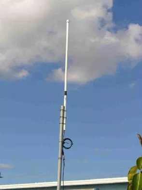
Monopole antenna are ideally about one-quarter of a wavelength in length.
Dipole antennas are ideally about one-half of a wavelength in length.
C
o
m
p
a
r
i
s
o
n
o
f
W
i
r
e
d
S
y
s
t
e
m
s
w
i
t
h
W
i
r
e
l
e
s
s
S
y
s
t
e
m
s
6
Wireless systems using antennas will always be better (lower loss)
than wired (transmission line) systems for large distances.
C
o
m
p
a
r
i
s
o
n
o
f
W
i
r
e
d
S
y
s
t
e
m
s
w
i
t
h
W
i
r
e
l
e
s
s
S
y
s
t
e
m
s
(
c
o
n
t
.
)
7
8
8
RG59
1
G
H
z
Single Mode
Two Dipoles
34m Dish+Dipole
A
t
t
e
n
u
a
t
i
o
n
i
n
d
B
C
o
m
p
a
r
i
s
o
n
o
f
W
i
r
e
d
S
y
s
t
e
m
s
w
i
t
h
W
i
r
e
l
e
s
s
S
y
s
t
e
m
s
(
c
o
n
t
.
)
V
e
c
t
o
r
W
a
v
e
E
q
u
a
t
i
o
n
Start with Maxwell’s equations in the phasor domain:
Faraday’s law
Ampere’s law
Assume
free space
:
We then have:
Ohm’s law:
9
V
e
c
t
o
r
W
a
v
e
E
q
u
a
t
i
o
n
(
c
o
n
t
.
)
Take the curl of the first equation and then substitute the
second equation into the first one:
“Vector wave equation”
Define:
Then
Wavenumber of free space [
rad/m
]
10
V
e
c
t
o
r
H
e
l
m
h
o
l
t
z
E
q
u
a
t
i
o
n
Recall the vector Laplacian identity:
Hence, we have
Also, from the electric Gauss law we have (in free space):
11
Hence, we have:
Vector Helmholtz equation
Recall the property of the vector Laplacian in rectangular coordinates:
Taking the
x
component of the vector Helmholtz equation, we have
Scalar Helmholtz equation
12
R
e
m
i
n
d
e
r
:
This identity only holds in
rectangular coordinates.
V
e
c
t
o
r
H
e
l
m
h
o
l
t
z
E
q
u
a
t
i
o
n
(
c
o
n
t
.
)
P
l
a
n
e
W
a
v
e
F
i
e
l
d
Assume
Then
or
Solution:
The electric field is
polarized
in the
x
direction, and
the wave is
propagating
(traveling) in the
z
direction.
For wave traveling in the
negative
z
direction:
13
N
o
t
e
:
The electric field is constant
in the
z
= 0
plane.
where
For a plane wave traveling in a lossless
dielectric
medium
(does not have to be free space):
(wavenumber of dielectric medium)
P
l
a
n
e
W
a
v
e
F
i
e
l
d
(
c
o
n
t
.
)
14
L
o
s
s
l
e
s
s
D
i
e
l
e
c
t
r
i
c
M
e
d
i
u
m
:
The electric field of a plane wave in a lossless medium propagates in
z
exactly as does the voltage on a lossless transmission line (filled with
the same material):
Transmission Line:
P
l
a
n
e
W
a
v
e
F
i
e
l
d
(
c
o
n
t
.
)
15
C
o
m
p
a
r
i
s
o
n
b
e
t
w
e
e
n
p
l
a
n
e
w
a
v
e
a
n
d
w
a
v
e
o
n
a
l
o
s
s
l
e
s
s
t
r
a
n
s
m
i
s
s
i
o
n
l
i
n
e
Plane Wave:
They have the same wavenumber!
The
H
field is found from:
so
16
P
l
a
n
e
W
a
v
e
F
i
e
l
d
(
c
o
n
t
.
)
I
n
t
r
i
n
s
i
c
I
m
p
e
d
a
n
c
e
We then have
Hence
where
(intrinsic impedance of the medium)
Intrinsic impedance of free-space:
17
so
P
o
y
n
t
i
n
g
V
e
c
t
o
r
The complex Poynting vector is given by
Hence, we have:
18
(no VARS)
For a wave traveling in a
lossless
dielectric medium:
N
o
t
e
:
k
and
are
real here
(lossless medium).
P
h
a
s
e
V
e
l
o
c
i
t
y
From our previous discussion on phase velocity for transmission
lines, we know that for a wave on a transmission line:
Hence, for a plane wave in a lossless dielectric medium (letting
=
k
):
(speed of light in the dielectric material)
so
N
o
t
e
s
:
All plane waves travel at the same speed in a lossless medium, regardless of the frequency.
This implies that there is no dispersion in a lossless medium, which in turn implies that there is no
distortion of the signal.
The phase velocity of a plane wave in a lossless medium is the same as that of a wave on a lossless
transmission line that is filled with the same material.
19
W
a
v
e
l
e
n
g
t
h
From our previous discussion on wavelength for transmission lines,
we know that
Hence, we have
For free space:
20
Hence, for a plane wave in a lossless dielectric medium (letting
=
k
):
S
u
m
m
a
r
y
(
L
o
s
s
l
e
s
s
C
a
s
e
)
21
L
o
s
s
y
M
e
d
i
u
m
Return to Maxwell’s equations:
Assume Ohm’s law:
Ampere’s law:
We define an
effective (complex) permittivity
c
that accounts for
conductivity
:
22
Set
Maxwell’s equations then become:
The lossy form is exactly the same as we have for the
lossless
case, with
Hence, we have for a lossy medium:
(complex)
(complex)
23
L
o
s
s
y
M
e
d
i
u
m
(
c
o
n
t
.
)
Lossy
Lossless
Examine the wavenumber:
Denote:
Compare with lossy TL:
24
L
o
s
s
y
M
e
d
i
u
m
(
c
o
n
t
.
)
25
L
o
s
s
y
M
e
d
i
u
m
(
c
o
n
t
.
)
The “depth of penetration”
d
p
is defined.
26
(choose
E
0
= 1
)
L
o
s
s
y
M
e
d
i
u
m
(
c
o
n
t
.
)
The complex Poynting vector is
27
L
o
s
s
y
M
e
d
i
u
m
(
c
o
n
t
.
)
N
o
t
e
:
T
h
e
a
n
g
l
e
b
e
t
w
e
e
n
t
h
e
E
x
a
n
d
H
y
p
h
a
s
o
r
s
i
s
.
28
L
o
s
s
y
M
e
d
i
u
m
(
c
o
n
t
.
)
S
u
m
m
a
r
y
f
o
r
D
e
p
t
h
o
f
P
e
n
e
t
r
a
t
i
o
n
F
o
r
m
u
l
a
:
E
x
a
m
p
l
e
O
c
e
a
n
w
a
t
e
r
:
Assume
f
= 2.0
GHz:
(These values are fairly constant up through
low microwave frequencies.)
29
E
x
a
m
p
l
e
(
c
o
n
t
.
)
f
d
p
[m]
1 [Hz] 251.6
10 [Hz] 79.6
100 [Hz] 25.2
1 [kHz] 7.96
10 [kHz] 2.52
100 [kHz] 0.796
1 [MHz] 0.262
10 [MHz] 0.080
100 [MHz] 0.0262
1.0 [GHz] 0.013
10.0 [GHz] 0.012
100 [GHz] 0.012
The depth of penetration
into ocean water is shown
for various frequencies.
30
N
o
t
e
:
The relative permittivity
of water starts
changing at very high
frequencies (above
about 2GHz), but this is
ignored here.
L
o
s
s
T
a
n
g
e
n
t
31
Recall:
To be more general:
Sometimes we write:
P
r
a
c
t
i
c
a
l
n
o
t
e
s
o
n
l
o
s
s
t
a
n
g
e
n
t
:
32
For some materials (mostly good conductors), it is the
conductivity
that is approximately
constant with frequency.
Ocean water:
4 [S/m]
For other materials (mostly good insulators), it is the
loss tangent
that is approximately
constant with frequency. In this case the effective permittivity is mainly due to molecular
loss effects.
Teflon:
tan
0.001
L
o
s
s
T
a
n
g
e
n
t
(
c
o
n
t
.
)
L
o
w
-
L
o
s
s
L
i
m
i
t
:
t
a
n
<
<
1
We approximate the wavenumber for
small
loss tangent:
33
(The derivation is omitted.)
I
n
t
h
e
l
o
w
-
l
o
s
s
l
i
m
i
t
,
t
h
e
d
e
p
t
h
o
f
p
e
n
e
t
r
a
t
i
o
n
i
s
i
n
d
e
p
e
n
d
e
n
t
o
f
f
r
e
q
u
e
n
c
y
.
f
d
p
[m] tan
1 [Hz] 251.6 8.88
10
8
10 [Hz] 79.6 8.88
10
7
100 [Hz] 25.2 8.88
10
6
1 [kHz] 7.96 8.88
10
5
10 [kHz] 2.52 8.88
10
4
100 [kHz] 0.796 8.88
10
3
1 [MHz] 0.262 888
10 [MHz] 0.080 88.8
100 [MHz] 0.0262 8.88
1.0 [GHz] 0.013 0.888
10.0 [GHz] 0.012 0.0888
100 [GHz] 0.012 0.00888
Ocean water
34
“Low-loss” region
O
c
e
a
n
W
a
t
e
r
D
i
s
t
i
l
l
e
d
W
a
t
e
r
35
N
o
t
e
:
For pure distilled water,
the effective conductivity
is due entirely to
molecular loss effects,
since pure water is almost
a perfect insulator (no
ions to carry current as for
ocean water).
A
p
p
e
n
d
i
x
:
S
u
m
m
a
r
y
o
f
F
o
r
m
u
l
a
s
36
L
o
s
s
l
e
s
s
A
p
p
e
n
d
i
x
:
S
u
m
m
a
r
y
o
f
F
o
r
m
u
l
a
s
(
c
o
n
t
.
)
37
L
o
s
s
y
Introduction to plane waves, the electromagnetic spectrum, TV and radio spectrum, and a comparison of wired and wireless systems. Discusses the properties and applications of various frequency ranges within the electromagnetic spectrum. Highlights the efficiency of wireless systems over wired systems for long-distance communication.

Download Presentation

Please find below an Image/Link to download the presentation.
The content on the website is provided AS IS for your information and personal use only. It may not be sold, licensed, or shared on other websites without obtaining consent from the author. Download presentation by click this link. If you encounter any issues during the download, it is possible that the publisher has removed the file from their server.
E N D
Presentation Transcript
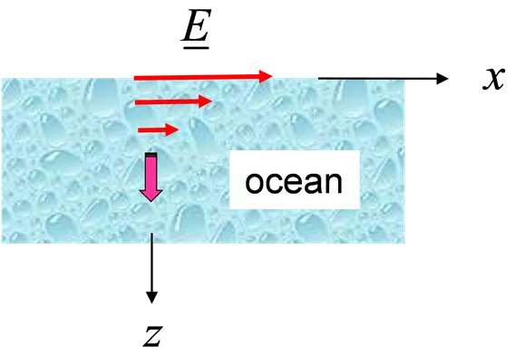
ECE 3317 Applied Electromagnetic Waves Prof. David R. Jackson Fall 2023 Notes 15 Plane Waves E x ocean z 1
Introduction to Plane Waves A plane wave is the simplest solution to Maxwell s equations for a wave that travels through free space. The wave does not require any conductors it exists in free space. A plane wave is a good model for radiation from an antenna, if we are far enough away from the antenna. x E S z H 1 2 1 2 ( ) = E H = * * y z S E H x 2
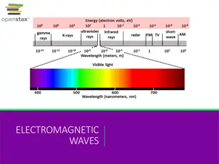
The Electromagnetic Spectrum = / c f 0 File:EM Spectrum Properties edit.svg http://en.wikipedia.org/wiki/Electromagnetic_spectrum 3
The Electromagnetic Spectrum (cont.) Source Frequency Wavelength U.S. AC Power 60 Hz 5000 km ELF Submarine Communications 500 Hz 600 km AM radio (KTRH) 740 kHz 405 m TV ch. 2 (VHF) 60 MHz 5 m FM radio (Sunny 99.1) 99.1 MHz 3 m TV PBS ch. 8 (VHF ch 8) 183 MHz 1.6 m TV KPRC ch. 2 (UHF ch. 35) 599 MHz 50 cm Cell Phone (4G) 1.9 GHz 16 cm -wave oven 2.45 GHz 12 cm Police radar (X-band) 10.5 GHz 2.85 cm Cell Phone (Verizon 5G mmWave) 28 GHz 1.1 cm THz 1000 GHz 0.3 mm 5 1014 [Hz] 0.60 m Light X-ray 1018 [Hz] 3 = / c f 0cm Note: 30/ GHz f 0 4
TV and Radio Spectrum AM Radio: 520-1610 kHz VHF TV: 55-216 MHz (channels 2-13) Band I : 55-88 MHz (channels 2-6) Band III: 174-216 MHz (channels 7-13) FM Radio: (Band II) 88-108 MHz UHF TV: 470-806 MHz (channels 14-69) Digital TV broadcast takes place primarily in UHF and VHF Bands I & III. Note: Monopole antenna are ideally about one-quarter of a wavelength in length. Dipole antennas are ideally about one-half of a wavelength in length. 5
Comparison of Wired Systems with Wireless Systems Wireless systems using antennas will always be better (lower loss) than wired (transmission line) systems for large distances. 2 1/ r Power loss from antenna broadcast: (always better for very large r) 2 r e Power loss from waveguiding system: Antenna r B A Transmission line system 6
Comparison of Wired Systems with Wireless Systems (cont.) Comparison of Two Functions 1 1 2 r e 0.1 = 0.1 np/m 0.01 f x ( ) 3 1 10 g x ( ) 4 1 10 2 1/ r 5 1 10 0.000001 6 1 10 103 104 1 1 10 100 x 1 1 10000 r [meters] 7
Comparison of Wired Systems with Wireless Systems (cont.) 1 GHz Attenuation in dB Single Mode Two Dipoles RG59 34m Dish+Dipole Distance 1 m 10 m 100 m 1 km 10 km 100 km 1000 km 10,000 km 100,000 km 1,000,000 km 10,000,000 km 100,000,000 km Coax 0.4 4 40 400 4000 - - - - - - - Fiber 0.0003 0.003 0.03 0.3 3 30 300 3000 - - - - Wireless 28.2 48.2 68.2 88.2 108.2 128.2 148.2 168.2 188.2 208.2 228.2 248.2 Wireless - - - 39.3 59.3 79.3 99.3 119.3 139.3 159.3 179.3 199.3 8 8
Vector Wave Equation Start with Maxwell s equations in the phasor domain: = = E H j + H Faraday s law J j E Ampere s law Assume free space: = = = = 0 J E , Ohm s law: 0 0 We then have: = = E H j H 0 j E 0 9
Vector Wave Equation (cont.) = = E H j H 0 j E 0 Take the curl of the first equation and then substitute the second equation into the first one: ( ) ( ( ) = = E j H 0 ) j j E 0 0 Define: k Wavenumber of free space [rad/m] 0 0 0 Then ( ) = 2 0 0 E k E Vector wave equation 10
Vector Helmholtz Equation ( ) = 2 0 0 E k E Recall the vector Laplacian identity: ( ) ( ) 2V V V Hence, we have ( ) = 2 2 0 0 E E k E Also, from the electric Gauss law we have (in free space): 1 1 = = = 0 E D v 0 0 11
Vector Helmholtz Equation (cont.) Hence, we have: + = 2 2 0 0 E k E Vector Helmholtz equation Recall the property of the vector Laplacian in rectangular coordinates: Reminder: = + + 2 2 2 2 x y z V V V V This identity only holds in rectangular coordinates. x y z Taking the x component of the vector Helmholtz equation, we have + = 2 2 0 0 E k E Scalar Helmholtz equation x x 12
Plane Wave Field z = x E z ( ) E Assume x The electric field is polarized in the x direction, and the wave is propagating (traveling) in the z direction. y Then E + = 2 2 0 0 E k E x x x or 2 2 2 E x E y E z + + + = 2 0 0 k E x x x Note: x 2 2 2 The electric field is constant in the z = 0 plane. 2 d E dz + = 2 0 0 k E x x 2 For wave traveling in the negative z direction: E e+ = jk z ( ) E z E e = jk z 0 ( ) E z = Solution: ( ) k 0 0 x 0 x 0 0 0 13
Plane Wave Field (cont.) Lossless Dielectric Medium: For a plane wave traveling in a lossless dielectric medium (does not have to be free space): E e = jkz ( ) E z 0 x where = = k k (wavenumber of dielectric medium) 0 r r = = 0 r 0 r 14
Plane Wave Field (cont.) Comparison between plane wave and wave on a lossless transmission line E e = jkz ( ) E z Plane Wave: 0 x j z = ( ) V z V e Transmission Line: 0 The electric field of a plane wave in a lossless medium propagates in z exactly as does the voltage on a lossless transmission line (filled with the same material): LC = = = k They have the same wavenumber! 15
Plane Wave Field (cont.) E e = jkz ( ) E z 0 x The H field is found from: = E j H so 1 ( ) ( ) z = x E H x j x y z 1 d E dz = y x = E j x y z 1 E E E ( ) = ( y ) jk E x y z x j 16
Intrinsic Impedance k k = = y H E H E We then have so x y x Hence E H = = = = x k y where = (intrinsic impedance of the medium) r 0 r = 7 4 10 [H/m] ( ) exact before 2019 0 1 = 12 8.854 10 [F/m] 0 2 c Intrinsic impedance of free-space: 0 2.99792458 10 [m/s] ( 8 ) c exact = 376.730313 [ ] 0 1 = c 0 0 0 0 17
Poynting Vector For a wave traveling in a lossless dielectric medium: = jkz x E e E Note: 0 k and are real here (lossless medium). 1 = jkz y H E e 0 1 2 ( ) = * S E H The complex Poynting vector is given by Hence, we have: * 1 2 1 2 1 2 E ( ) 2 = jkz jkz S z E e e 0 E 0 = 2 0 z [VA/m ] S (no VARS) 2 ( )( ) + = * 0 jkz jkz z E e E e 0 2 E ( ) t ( ) S = = 0 2 S z Re [W/m ] 2 = z E 2 0 18
Phase Velocity From our previous discussion on phase velocity for transmission lines, we know that for a wave on a transmission line: = p v Hence, for a plane wave in a lossless dielectric medium (letting = k): 1 = = = p v k so 1 = = v c (speed of light in the dielectric material) p d Notes: All plane waves travel at the same speed in a lossless medium, regardless of the frequency. This implies that there is no dispersion in a lossless medium, which in turn implies that there is no distortion of the signal. The phase velocity of a plane wave in a lossless medium is the same as that of a wave on a lossless transmission line that is filled with the same material. 19
Wavelength From our previous discussion on wavelength for transmission lines, we know that 2 g = Hence, for a plane wave in a lossless dielectric medium (letting = k): 2 2 2 f 1 / c c f = = = = = = = = 0 d f g d k 2 f r r r r Hence, we have = = 0 g d r r = For free space: / c f 0 20
Summary (Lossless Case) z = jkz E E e 0 x S 1 = jkz H E e 0 y y 2 H E E = 0 S x z 2 c = = = v c = = k 0 p d g d r r r r = = r = 376.730313 [ ] 0 0 0 r 0 21
Lossy Medium Return to Maxwell s equations: E = = E H j + H x J j E Ocean = J E Assume Ohm s law: Ampere s law: z = = + H E j E E ( ) + j We define an effective (complex) permittivity c that accounts for conductivity: = + j j j Set c c 22
Lossy Medium (cont.) Maxwell s equations then become: = = E H j H E = = E H j H j j E c Lossy Lossless The lossy form is exactly the same as we have for the lossless case, with c Hence, we have for a lossy medium: = = jkz E E e k (complex) c 0 x 1 = jkz H E e = (complex) 0 y c 23
Lossy Medium (cont.) = k Examine the wavenumber: = j c c Reminder about principal branch: c k = = /2 j j z z e z e 0 0 k k = k k jk Denote: k z = = jkz jk z E E e E e e 0 0 x k k Compare with lossy TL: 24
Lossy Medium (cont.) ( ) z ( ) ( ) k z k z k z = = + jk z xz t E , cos E E e e E t e 0 0 0 x = j E E e 0 0 0 t = 0 g ( ) xz E ,0 k z E e 0 z 2 k = g 25
Lossy Medium (cont.) ( ) z k z = jk z E E e e 0 x (choose E0 = 1) ( ) z 1 E x k z e e 1 0.37 z d p The depth of penetration dpis defined. k 1/ d k d = 1 p p 26
Lossy Medium (cont.) k z = jk z E E e e 0 x = = j e 1 c k z = jk z H E e e 0 y Note: The angle between the Ex and Hy phasors is . The complex Poynting vector is 2 2 E E 1 2 1 2 ( ) k z k z = = = = * * y 2 2 j 0 0 z z z S E H E H e e e x * 2 2 1 ( ) z z S 2 E 2k z e ( ) k z = = 2 0 Re cos S t S e z z 2 e = 2 0.14 z k = 1/ d p 27
Lossy Medium (cont.) Summary for Depth of Penetration Formula: k 1/ d p ( ) = = Im( ) k k jk k k = = = / k k k 0 0 0 c c rc = = , c j j c rc r 0 0 28
Example r = = = 81 4 [S/m] Ocean water: (These values are fairly constant up through low microwave frequencies.) 0 Assume f= 2.0 GHz: ( ) ( ) = 081 35.95 [F/m] j c = = j j ( ) 0 c r = 81 35.95 j 0 rc ( ) = = = = k k 386.022 81.816 [1/m] k j 0 0 0 0 c rc rc k = 386.022 [rad/m] k d = = 0.01222 [m] 1/ d p p k = 81.816 [nepers/m] = 2 / g = k 0.01628 [m] g 29
Example (cont.) fdp [m] 1 [Hz] 251.6 The depth of penetration into ocean water is shown for various frequencies. 10 [Hz] 79.6 100 [Hz] 25.2 1 [kHz] 7.96 r = = = 81 4 [S/m] Note: 10 [kHz] 2.52 The relative permittivity of water starts changing at very high frequencies (above about 2GHz), but this is ignored here. 100 [kHz] 0.796 1 [MHz] 0.262 0 10 [MHz] 0.080 100 [MHz] 0.0262 k = 1/ d p 1.0 [GHz] 0.013 10.0 [GHz] 0.012 100 [GHz] 0.012 30
Loss Tangent Recall: = j = = conductivity of dielectric material c d To be more general: = = (accounts for actual conductivity + atomic and molecular loss effects) conductivity of dielectric material effective = eff d = tan 0 r Sometimes we write: r r = = = / j j 0 rc c c r r = = = tan , = = , r 0 31
Loss Tangent (cont.) Practical notes on loss tangent: For some materials (mostly good conductors), it is the conductivity that is approximately constant with frequency. Ocean water: 4 [S/m] For other materials (mostly good insulators), it is the loss tangent that is approximately constant with frequency. In this case the effective permittivity is mainly due to molecular loss effects. Teflon: tan 0.001 32
Low-Loss Limit: tan << 1 We approximate the wavenumber for small loss tangent: (The derivation is omitted.) 2 ( ) tan 1 d p 0 In the low-loss limit, the depth of penetration is independent of frequency. 33
Ocean Water fdp [m] tan Ocean water 1 [Hz] 251.6 8.88 108 10 [Hz] 79.6 8.88 107 = tan 100 [Hz] 25.2 8.88 106 0 r 1 [kHz] 7.96 8.88 105 10 [kHz] 2.52 8.88 104 r = = = 81 4 [S/m] 100 [kHz] 0.796 8.88 103 1 [MHz] 0.262 888 0 10 [MHz] 0.080 88.8 100 [MHz] 0.0262 8.88 1.0 [GHz] 0.013 0.888 10.0 [GHz] 0.012 0.0888 Low-loss region tan 100 [GHz] 0.012 0.00888 1 34
Distilled Water Complex Relative Permittivity for Pure (Distilled) Water j r r = = = c j r r = = , eff r rc 0 0 0 r = = tan Note: r r For pure distilled water, the effective conductivity is due entirely to molecular loss effects, since pure water is almost a perfect insulator (no ions to carry current as for ocean water). r Frequency [GHz] 35
Appendix: Summary of Formulas Lossless E e = jkz ( ) E z 0 x = = 0 g d r r = k c = c E H = d x r r y c f = = = r 0 0 r = v c = p d 376.730313[ ] 0 0 0 36
Appendix: Summary of Formulas (cont.) Lossy E e = jkz ( ) E z 0 x = j = k k jk = k c c k 1/ = d E H j = x p c y 2 k = = tan = g 0 r = c 37


")


")
")

")

")

")
")
")


")

")
")
")
")
")
")

")

")


")