Wireless Networking - III: MIMO and Beamforming

Wireless Networking - III:
MIMO and Beamforming
CS 655: Wireless and Mobile Computing
Parth H. Pathak
8
0
2
.
1
1
P
H
Y
a
n
d
M
A
C
2
MAC:
CSMA/CA and wideband
medium access
PHY-I:
OFDM and modulation
PHY-II:
MIMO and beamforming
W
i
r
e
l
e
s
s
n
e
t
w
o
r
k
i
n
g
-
I
Today’s agenda
•
MIMO overview
•
MIMO rate adaptation
•
MIMO energy consumption
•
Beamforming
•
MU-MIMO and user selection
3
W
i
r
e
l
e
s
s
C
a
p
a
c
i
t
y
Wireless channel capacity – Shannon’s theorem
4
B = bandwidth (Hz)
S/N = Signal to noise ratio (SNR)
How can we increase the capacity (achievable data rate/speed) of a
wireless link/channel?
How about we simply increase channel bandwidth (B)?
Problem: spectrum scarcity – Nearly impossible to find usable bandwidth, frequency
W
i
r
e
l
e
s
s
C
a
p
a
c
i
t
y
Wireless channel capacity – Shannon’s theorem
5
B = bandwidth (Hz)
S/N = Signal to noise ratio (SNR)
How can we increase the capacity (achievable data rate/speed) of a
wireless link/channel?
How about increasing SNR? Increase the signal power to increase S?
Problem: increasing transmission
power will also increase your
interference to other links
More channel sharing, more
collisions, lower speeds
The quest for more wireless channel capacity –
by far the most important research problem
Increase spectral efficiency -> bits/sec/Hz
M
u
l
t
i
p
l
e
A
n
t
e
n
n
a
S
y
s
t
e
m
s
Wireless devices can be equipped with multiple antennas
•
Can multiple antennas increase the achievable capacity?
Multiple antenna systems
•
Early research in 1990s showed huge capacity gains
•
Practical systems developed in early 2000s
•
Commonly used in current WiFi, LTE, WiMax systems
Capacity gains
•
If only one end point (Tx or Rx) has multiple antennas
o
Linear increase in SNR
without increasing transmission power
•
If both Tx and Rx have multiple antennas
o
Linear increase in capacity
for every pair of Tx, Rx antenna
6
M
I
M
O
7
Tx
Rx
Tx
Rx
Tx
Rx
Tx
Rx
SISO (Single Input Single Output)
MISO (Multiple Input Single Output)
SIMO (Single Input Multiple Output)
MIMO (Multiple Input Multiple Output)
All antenna utilize the same frequency and channel
S
p
a
t
i
a
l
D
i
v
e
r
s
i
t
y
Paths between antennas
•
Multiple antennas enable multiple paths between Tx and Rx
•
These paths observe independent fading
Spatial paths
•
Independent paths between antennas can be exploited to increase gain
Shannon’s capacity
•
Capacity gain through spatial diversity/freedom
8
C
h
a
n
n
e
l
M
a
t
r
i
x
9
Received signal
Channel matrix/vector
Transmitted signal
noise
OFDM with S subcarriers,
where
Amplitude
Phase
C
h
a
n
n
e
l
M
a
t
r
i
x
10
H
is a
M x N x S
matrix
Where
M
= number of Tx antenna
N
= number of Rx antenna
S
= number of subcarriers
OFDM with S subcarriers,
M
I
M
O
T
e
c
h
n
i
q
u
e
s
[
1
]
How to take advantage of multiple antennas at Tx, Rx or both?
11
Multi-antenna
systems
MISO/SIMO
Selection
Combining (SEL)
Maximal-Ratio
Combining (MRC)
MIMO
Spatial multiplexing
Direct-mapped
MIMO
Precoded
MIMO
S
I
M
O
SIMO – Single Input Multiple Output
•
Each receiving antenna receives a copy of the transmitted signal
•
Signal variation can be measured at the receiver using the H matrix
How to combine the received signal at the receiver?
12
MIMO notation (M x N)
where
M is number of transmit antenna
N is number of receive antenna
S
I
M
O
Receiver diversity
techniques
1.
Selection Combining (SEL)
•
Pick the antenna with the strongest SNR
•
Used in early generation 802.11a/g devices
•
Does not take advantage of other available antennas
13
S
I
M
O
Receiver diversity techniques
2.
Maximal Ratio Combining (MRC)
•
Use signal available through each Rx antenna
•
Signal combining
o
Weight the signal of each antenna using its SNR
o
Amplify useful signal and reduce noise
o
Sum the weighted signals
•
Challenges?
o
Each signal received on different path (separate H
mn
)
o
Phase is different for each received signal
o
Align the phase through a reference before combining the signal
14
S
E
L
v
s
.
M
R
C
802.11n link with 1x3 configuration
•
Each Rx antenna (A, B, C) observes independent channel fading
•
SEL selects B – best SNR
•
MRC (for AB and ABC) substantially improves the SNR
•
MRC more complex to implement but higher performance gain compared to
SEL
15
[1]
M
I
S
O
Transmit diversity techniques
1.
Selection Combining (SEL)
•
Pick the best (highest SNR) antenna to send the signal
2.
Maximal Ratio Combining (MRC)
•
Transmitter precodes the signal
o
Apply more power to the antenna path which provides higher SNR
o
Delay the phase in such as way that transmitted signal from all antennas combine
constructively at the receiver
How to know which antenna is the best?
16
M
I
S
O
Transmit diversity techniques
•
Requires feedback
Channel feedback from receiver
•
Transmitter sends data to receiver
•
Receiver observe the channel matrix for each spatial path
•
Receiver sends the measured channel matrix back to transmitter
•
Transmitter uses the feedback for SEL or MRC
Reciprocity
•
Transmitter measures the channel matrix when it receives a packets from
receiver
•
Calibration required to account for differences (different hardware, number
of antennas)
17
M
I
M
O
a
n
d
C
a
p
a
c
i
t
y
18
[1]
M
I
M
O
a
n
d
C
a
p
a
c
i
t
y
19
[1]
M
I
M
O
a
n
d
C
a
p
a
c
i
t
y
20
[1]
M
I
M
O
a
n
d
C
a
p
a
c
i
t
y
21
[1]
M
I
M
O
a
n
d
C
a
p
a
c
i
t
y
22
[1]
M
I
M
O
M x N antenna systems
•
Diversity techniques simply increase SNR
Spatial multiplexing
•
Use the independent spatial paths enabled by M x N antennas to send
parallel streams of data (referred as spatial streams)
•
Each spatial stream carries different data
•
All spatial streams occupy same frequency channel and time
•
Number of spatial streams can be min(M, N)
•
Parallel spatial paths over the same frequency channel
•
Min(M, N) fold increase in capacity
23
M
I
M
O
s
p
a
t
i
a
l
m
u
l
t
i
p
l
e
x
i
n
g
Direct Mapped MIMO
•
Transmitter divides the transmit power equally among all spatial streams
•
Each spatial stream transmitted out of one transmit antenna
•
802.11n/ac devices use training fields at the start of the frame
•
Receiver uses the training fields to estimate H
•
Use H to decode the transmitted data over each stream
•
Two types of common receivers
o
Zero forcing (ZF) receivers
o
Minimum Mean Square Error (MMSE) receivers
24
M
I
M
O
s
p
a
t
i
a
l
m
u
l
t
i
p
l
e
x
i
n
g
Precoded MIMO
•
Direct mapped MIMO makes decoding to be completely receiver’s
responsibility
•
In precoded MIMO, transmitter can use the channel matrix to precode the
data before transmitting over the antennas
•
Requires explicit channel feedback from the receiver
•
Improves receiver’s ability to untangle the spatial streams and decode data
Precoded vs. direct mapped
•
Precoded MIMO performs better (closer to maximum achievable capacity)
•
Direct mapped simpler to implement
•
802.11n/ac devices can use all variations of MIMO described here
25
M
I
M
O
i
n
8
0
2
.
1
1
n
26
Single Stream (SS) mode -
uses transmit and/or
receiver diversity
techniques
Double Stream (DS) mode –
uses spatial multiplexing
M
I
M
O
i
n
8
0
2
.
1
1
a
c
27
8
0
2
.
1
1
P
H
Y
a
n
d
M
A
C
28
MAC:
CSMA/CA and wideband
medium access
PHY-I:
OFDM and modulation
PHY-II:
MIMO and beamforming
W
i
r
e
l
e
s
s
n
e
t
w
o
r
k
i
n
g
-
I
Today’s agenda
•
MIMO overview
•
MIMO rate adaptation
•
MIMO energy consumption
•
Beamforming
•
MU-MIMO and user selection
29
R
a
t
e
a
d
a
p
t
a
t
i
o
n
w
i
t
h
M
I
M
O
MIMO and rate adaptation
•
Use of spatial streams further complicates rate adaptation
How to design an ideal rate adaptation scheme?
Dynamically choose rate based on many factors
•
Before MIMO
o
RSS, SNR
o
Channel quality
o
Frame loss (not collisions)
o
PHY indicators – BER
•
With MIMO
o
Number of spatial streams
o
Diversity techniques or spatial multiplexing
Have to address questions like
•
Choose a higher modulation order (e.g. 64QAM) with 1 spatial stream or
lower modulation order (16QAM) with 2 spatial streams?
30
R
a
t
e
A
d
a
p
t
a
t
i
o
n
w
i
t
h
M
I
M
O
MIMO Rate Adaptation (MiRA) [2]
•
802.11n specific
MiRA
•
Identifies that pre-MIMO rate adaptation algorithms are not suitable for
MIMO
•
Shows that rate increase/decrease can be non-monotonic, requires switching
back and forth between number of spatial streams
31
M
i
R
A
R
a
t
e
S
p
a
c
e
32
Single Stream (SS) mode -
uses transmit and/or
receiver diversity
techniques
Double Stream (DS) mode –
uses spatial multiplexing
802.11n rates with 1 or 2 spatial streams
8
0
2
.
1
1
n
F
r
a
m
e
E
r
r
o
r
R
a
t
e
MiRA utilizes frame loss as a channel quality indicator
•
Compares data rate and goodput
802.11n frame aggregation
•
11n/ac utilizes large MAC frames (A-MPDU) where each frame contains
multiple MAC frames (MPDU)
•
A-MPDU – Aggregate MAC Protocol Data Unit
MiRA uses SFER to measure frame loss in presence of aggregation
•
SFER – Sub-Frame Error Rate
•
Percentage of sub-frames lost
•
Also accounts for loss of A-MPDU
33
What is the
advantage of frame
aggregation?
M
i
R
A
C
a
s
e
S
t
u
d
y
34
Current rate adaptation algorithms not sufficient for 802.11n MIMO links
[2]
M
i
R
A
C
a
s
e
S
t
u
d
y
Why RRAA, SampleRate and other algorithms perform worse?
•
They assume monotonic relationship between rate and SFER
•
Increase/decrease the rate by probing the higher/lower rate
But with MIMO
•
Rates and SFER are non-monotonic
35
[2]
R
a
t
e
a
n
d
F
r
a
m
e
L
o
s
s
R
a
t
e
How to adapt rate if frame loss not monotonous with data rate?
•
Basis of most conventional algorithms
•
Monotonicity still holds within one (SS) or two (DS) spatial stream mode
•
Challenge – how and when to switch between SS and DS rates?
36
[2]
M
i
R
A
a
l
g
o
r
i
t
h
m
MiRA relies on goodput estimate
•
Expected goodput = frame loss rate x data rate
For the current rate r
•
Observe the goodput
G(r)
•
If measured goodput
G(r) <= G(r)
avg
– 2 G(r)
std
,
o
Start probing downward to a lower rate
•
Else
o
Start probing upward to a higher rate
Sequence of rates to probe
•
Probe the intra-mode rates first
37
Moving average
M
i
R
A
a
l
g
o
r
i
t
h
m
Candidate rates for probing
•
When probing upward,
o
Start by probing the immediate higher rate in the same mode
o
Probing within the same mode stops
•
When the next higher rate gives a goodput estimate smaller than the highest
goodput estimate obtained so far
•
If so, start inter-mode probing
•
Start by probing the lowest rate for which loss-free goodput estimate is higher than
the current goodput
•
Similar procedure followed while probing downward
o
Start by probing immediate lower rate within the same mode until the highest
goodput estimate so far is larger than the next lower rate
38
M
i
R
A
e
x
a
m
p
l
e
MiRA strategy
•
Favor intra-mode increase/decrease over inter-mode
•
Probe upward/downward within the same mode (SS or DS) until no better
rate can be found before changing mode
39
[2]
C
h
a
n
n
e
l
q
u
a
l
i
t
y
v
s
.
c
o
l
l
i
s
i
o
n
s
MIMO also changes how collisions can be detected
Frame aggregation in 802.11n
•
Difference in entire frame lost or some sub-frames lost
RTS/CTS
•
Relying on RTS to detect collision requires using RTC/CTS
•
With higher data rates of 802.11n, RTS/CTS is significant overhead
•
MiRA uses adaptive RTS/CTS
•
Send RTS before the frame if the transmission time of the frame (size/rate) is
higher than (k x time for RTS)
•
k = 1.5 is the cost/benefit ratio – avoid cases when retransmission at a high
data rate consumes lesser time than sending RTS
40
M
i
R
A
P
e
r
f
o
r
m
a
n
c
e
41
W
i
r
e
l
e
s
s
n
e
t
w
o
r
k
i
n
g
-
I
Today’s agenda
•
MIMO overview
•
MIMO rate adaptation
•
MIMO energy consumption
•
Beamforming
•
MU-MIMO and user selection
42
M
I
M
O
P
o
w
e
r
C
o
n
s
u
m
p
t
i
o
n
More antennas require more radio chains for signal processing
•
Increases the power consumption on devices
43
[3]
M
I
M
O
E
n
e
r
g
y
C
o
n
s
u
m
p
t
i
o
n
Calculated for Intel 802.11n chipset
44
[4]
M
I
M
O
v
s
.
C
h
a
n
n
e
l
w
i
d
t
h
MIMO
•
Increasing number of spatial streams by k gives k-fold increase in data rate
Channel width
•
Doubling the channel width doubles the data rate
Which technique is better in terms of energy consumption?
45
M
I
M
O
v
s
.
C
h
a
n
n
e
l
w
i
d
t
h
Increasing SS is a more energy-efficient alternative compared with doubling the
channel width for achieving the same percentage increase in throughput
46
Why?
[5]
W
i
r
e
l
e
s
s
n
e
t
w
o
r
k
i
n
g
-
I
Today’s agenda
•
MIMO overview
•
MIMO rate adaptation
•
MIMO energy consumption
•
Beamforming
•
MU-MIMO and user selection
47
O
m
n
i
-
d
i
r
e
c
t
i
o
n
a
l
a
n
t
e
n
n
a
Omni directional antenna
•
Commonly used in 802.11 WiFi networks
Advantages
•
Coverage in all directions
•
Simpler hardware design
Disadvantages
•
A large amount of radiated power is wasted
•
Can we concentrate the radiated transmission energy towards the intended
receivers?
o
Can increase SNR for intended receivers
o
Reduce interference to other devices
48
O
m
n
i
-
d
i
r
e
c
t
i
o
n
a
l
a
n
t
e
n
n
a
Directional antenna
•
Widely used in special purpose
applications
Advantages
•
Higher signal strength in desired direction
•
Reduced interference to other devices
Disadvantages
•
Coverage restricted to some direction
•
Costly - multiple antennas needed for omni
coverage, capacity (similar to sectors used
in cellular network base stations)
•
Solution – electronic beamforming
49
Av Dori - Image taken by Dori, Offentlig eiendom,
https://commons.wikimedia.org/w/index.php?curi
d=100638
B
e
a
m
f
o
r
m
i
n
g
Beamforming
•
Use omni-directional antennas to focus signal in specific direction
•
Exploit multiple antennas used for MIMO
50
B
e
a
m
f
o
r
m
i
n
g
Signal strength
•
Beamforming can increase the SNR in desired direction
•
Depending on number of antennas used, SNR gain can be very high
Rate over range effect
•
Beamforming can increase the range till a given data rate can be supported
51
MCS
9
8
7
6
5
4
3
2
1
0
Distance from AP
MCS
9
8
7
6
5
4
3
2
1
0
Distance from AP
B
e
a
m
f
o
r
m
i
n
g
Beamforming using multiple antenna
52
B
e
a
m
f
o
r
m
i
n
g
Beamforming
•
Constructive interference
•
When signal meet in phase, resultant signal strength increases
53
Higher signal
strength; 3x in an
ideal case
B
e
a
m
f
o
r
m
i
n
g
Beamforming
•
Destructive interference
•
When signal meet out of phase, resultant signal strength weakens
54
Lower signal strength
B
e
a
m
f
o
r
m
i
n
g
Beamforming
•
Use omni-directional antennas to focus signal in a specific direction
•
Change the phase of signal emitting from different antenna
•
Intelligent phase modification can result in beams in desired direction
55
Same frequency,
different phase
B
e
a
m
f
o
r
m
i
n
g
How can Tx form a beam towards Rx?
•
Actual received signal at Rx is mixture of direct and reflected multi-paths
•
Multi-path reflections also modify phase
•
Rx can measure Tx’s signal and provide channel measurement feedback to Tx
•
Explicit feedback more robust in capturing true channel state
56
What else affect the
phase of received signal
in practice?
B
e
a
m
f
o
r
m
i
n
g
Channel sounding procedure
•
Explicit feedback
•
Beamformer asks the beamformee to provide a feedback of channel
measurement
57
Request channel
measurement
Channel measurement
feedback
Data packets
(beamformed)
Calculate beam
steering matrix
Beamformer
(e.g. AP)
Beamformee
(e.g. laptop)
Measure channel
response
[6]
C
h
a
n
n
e
l
s
o
u
n
d
i
n
g
i
n
8
0
2
.
1
1
a
c
NULL Data Packet (NDP) Announcement
•
Beamformer first sends NDP announcement packet
•
Gain control over channel till channel sounding procedure is complete
•
Stations other than the beamformee will remain silent during the sounding
process
58
NULL data packet
announcement
Beamformer
Beamformee
C
h
a
n
n
e
l
s
o
u
n
d
i
n
g
i
n
8
0
2
.
1
1
a
c
NULL Data Packet (NDP)
•
Beamformer follows NDP announcement with NDP packet
•
As the name suggests, no data in included in NDP
•
NDP contains training fields/sequences which is used by the beamformee to
measure the channel response
59
NDP
announcement
Beamformer
Beamformee
NDP
C
h
a
n
n
e
l
s
o
u
n
d
i
n
g
i
n
8
0
2
.
1
1
a
c
Channel feedback – compressed beamforming feedback
•
Beamformee measure the channel response using NDP packet
•
Includes the measured channel response in feedback packet and sends it to
beamformer
•
Feedback is compressed before sending – resultant feedback is called
Compressed Beamforming Feedback (CBF)
60
NDP
announcement
Beamformer
Beamformee
NDP
Compressed
beamforming feedback
C
h
a
n
n
e
l
m
a
t
r
i
x
Channel State Information (CSI)
•
Also used as feedback for MIMO spatial multiplexing
•
Use NDP training fields to measure phase and amplitude of each OFDM
subcarriers, each Tx antenna and each Rx antenna
•
Challenge – the CSI matrix can be very large in size, especially for wider
channel widths (e.g. 160 MHz)
•
Frequent feedback necessary for accurate beamforming – high overhead
61
Number of
subcarriers
Number of Tx
antenna
Number of Rx
antenna
Feedback matrix
C
h
a
n
n
e
l
f
e
e
d
b
a
c
k
Compressed Beamforming Feedback (CBF)
•
Instead of sending the entire CSI matrix, beamformee transforms the matrix
through Singular Value Decomposition
•
Further compresses it using “Givens rotation” and quantization to yield CBF
o
Reduction in size over 120% compared to full CSI
•
After compression, beamformee sends the CBF to beamformer
Beamformer
•
After receiving the CBF, the beamformer calculates the steering matrix
•
The steering matrix is used to adjust the phase on each antenna such that
their transmitted signal meets constructively at the beamformee, essentially
creating a signal beam
62
W
i
r
e
l
e
s
s
n
e
t
w
o
r
k
i
n
g
-
I
Today’s agenda
•
MIMO overview
•
MIMO rate adaptation
•
MIMO energy consumption
•
Beamforming
•
MU-MIMO and user selection
63
M
u
l
t
i
-
U
s
e
r
B
e
a
m
f
o
r
m
i
n
g
Can the AP form beams to multiple clients at the same time?
Can it send separate data to each client at the same time?
64
B
A
C
M
u
l
t
i
-
U
s
e
r
M
I
M
O
(
M
U
-
M
I
M
O
)
MU-MIMO
•
Use multi-user beamforming to send data
•
AP can send separate spatial streams of data to different clients at the same
time
MIMO vs. MU-MIMO
65
Rx
Tx
Rx
2
Tx
Rx
1
Rx
3
Different color arrows indicate separate Spatial data streams
MIMO
MU-MIMO
M
U
-
M
I
M
O
MU-MIMO
•
A major change in wireless communication
paradigm
•
Sending separate data to different receivers
over the same frequency at the same time
Advantages in practice
•
In WLANs, APs typically have more antennas
(e.g. 4-8) than clients (e.g. 1-3)
•
Using MIMO, number of spatial streams can
be minimum of Tx and Rx antennas
•
With MU-MIMO, all antennas at the AP can
be used for serving different clients in
parallel
C
h
a
n
n
e
l
s
o
u
n
d
i
n
g
i
n
M
U
-
M
I
M
O
Channel feedback
•
Beamformer first sends NDP to one beamformee
•
Followed by BF report poll messages asking for channel feedback (CBF) from
other beamformees one after the other
67
NDPA
Beamformer
Beamformee - A
NDP
Channel
feedback
Beamformee - B
Beamformee - C
BF report
poll
Channel
feedback
BF report
poll
Channel
feedback
M
U
-
M
I
M
O
D
a
t
a
T
r
a
n
s
m
i
s
s
i
o
n
MU-MIMO MAC
•
Significant gains as AP doesn’t have to enter in carrier sense phase for every
frame
•
Multiple frames to different clients can be sent in channel access
68
Data - A
Beamformer
Data - A
Beamformee - A
ACK
Beamformee - B
Beamformee - C
Data - B
Data - C
ACK
ACK
Data - AP
ACK
Data - AP
ACK
[7]
C
h
a
l
l
e
n
g
e
s
i
n
M
U
-
M
I
M
O
Complexity of signal processing
•
Hardware design
•
802.11ac restricts MU-MIMO to downlink only (AP -> clients)
•
Maximum number of clients per AP MU-MIMO = 4
Interference
•
Inter-user interference if the clients of MU-MIMO are not far enough from
each other
•
Two techniques
o
Null steering
o
User grouping
69
I
n
t
e
r
f
e
r
e
n
c
e
i
n
M
U
-
M
I
M
O
Null steering
•
Calculate the beam steering matrix (Q) for each client such that signal is
maximum for the intended client and zero for all others
70
Rx
2
Tx
Rx
1
Rx
3
Q[Rx 1] * H[Rx 1] = high
Q[Rx 2] * H[Rx 1] = 0
Q[Rx 3] * H[Rx 1] = 0
Q[Rx 1] * H[Rx 2] = 0
Q[Rx 2] * H[Rx 2] = high
Q[Rx 3] * H[Rx 2] = 0
Q[Rx 1] * H[Rx 3] = 0
Q[Rx 2] * H[Rx 3] = 0
Q[Rx 3] * H[Rx 3] = high
Q[Rx i] = steering matrix to Rx i
H[Rx i] = channel matrix for Rx i
[6]
U
s
e
r
G
r
o
u
p
i
n
g
i
n
M
U
-
M
I
M
O
User Grouping
•
AP groups the client devices for MU-MIMO
•
Optimal groups are the ones where there is no interference between the
devices/users within the same group
•
AP serves users of only one group (downlink) at a time
71
B
A
C
E
D
F
G
B
A
C
E
D
F
G
U
s
e
r
G
r
o
u
p
i
n
g
802.11ac standard does not suggest any user grouping technique
Two categories of techniques proposed in research based on
•
Complete CSI feedback
•
Compressed CFB feedback
72
U
s
e
r
G
r
o
u
p
i
n
g
Optimal user grouping at AP
•
Request complete CSI (not the compressed CBF) from each user
•
Determine groups of users that do not interference with each other
•
Regroup further such that the sum of PHY data rate for each group is
maximized
•
Ensure data rate fairness among the groups
Computational complexity
•
Prohibitively large – even for today’s Aps
•
Overhead of complete CSI feedback more than MU-MIMO benefits
73
U
s
e
r
G
r
o
u
p
i
n
g
Incremental user selection
AP chooses the first user with best channel quality
Legacy-US: Greedy expansion of group [8]
•
Add the next user such that it does not interfere with the current user
•
Addition ensures high performance of the group
•
Continue until the maximum allowable number of users per group, and all
users are added to a group
74
U
s
e
r
G
r
o
u
p
i
n
g
OPUS protocol [8]
Incremental grouping with restricted feedback
How it works?
•
AP first receives CSI from the core user (the one included in NDP)
•
AP then calculates (signal) directions that are non-interfering to the core
user
•
It beamforms to these candidate signal directions and transmits BF report
poll asking for CSI
•
It then greedily picks the next user which maximizes group performance
75
U
s
e
r
G
r
o
u
p
i
n
g
In practice, user grouping needs to consider multiple factors other
than inter-group interference
Other factors?
•
Channel width
o
Users with different channel widths cannot be grouped
o
AP can transmit at one frequency and one bandwidth at a time
o
Grouping should consider channel widths available and supported by users
•
Data rate
o
Depending on channel conditions, it is possible that different users support different rates
at a time
o
MU-MIMO spatial streams can use different data rates
o
Grouping should consider how to maximize the total achievable data rate
76
U
s
e
r
G
r
o
u
p
i
n
g
Legacy-US: multiple clients (each with spatial stream) served in
parallel
SU-MIMO: one client served at a time
77
Legacy-US performs
really poorly (even
worse than SU-MIMO)
[9]
U
s
e
r
G
r
o
u
p
i
n
g
Challenge – how to estimate inter-user interference using CBF (no
CSI)?
New approach – MUSE [9]
Proves that higher correlation in CBF is an indication of inter-user
interference
•
Defines SINR through CBF correlation
The calculated SINR remains more or less constant for different
channel widths
•
Reason – total power in all subcarriers is constant
78
U
s
e
r
G
r
o
u
p
i
n
g
MUSE algorithm
SINR
•
Calculate SINR using CBF feedback from all users
Bandwidth – greedy strategy
•
Starts a greedy search from the highest bandwidth (e.g., 80MHz), and
considers only the users who can support that bandwidth
•
Sorts in descending order, the users based on their current throughput and
iteratively goes through the list to group the users that provide the highest
aggregate throughput with those already selected users.
•
At each iteration, it also ensures that user’s SINR is greater than a threshold
•
Search terminates when the group is complete, or when adding more users
to a group results in lower aggregate throughput than serving them in SU-
MIMO mode.
•
Search is repeated at lower bandwidths for only the incomplete groups, to
allow for more grouping opportunities.
79
M
U
S
E
P
e
r
f
o
r
m
a
n
c
e
Bandwidth adaptation is crucial in MU-MIMO user selection
Joint selection of users, rates and bandwidth is a complex and open research
problem
80
[9]
R
e
f
e
r
e
n
c
e
s
[1] Halperin, Daniel, Wenjun Hu, Anmol Sheth, and David Wetherall. "802.11 with multiple antennas for dummies." ACM SIGCOMM
Computer Communication Review 40, no. 1 (2010): 19-25.
[2] Pefkianakis, Ioannis, Yun Hu, Starsky HY Wong, Hao Yang, and Songwu Lu. "MIMO rate adaptation in 802.11 n wireless networks."
In Proceedings of the sixteenth annual international conference on Mobile computing and networking, pp. 257-268. ACM, 2010.
[3] Halperin, Daniel, Ben Greenstein, Anmol Sheth, and David Wetherall. "Demystifying 802.11 n power consumption." In Proceedings of the
2010 international conference on Power aware computing and systems, p. 1. 2010.
[4] Khan, Muhammad Owais, Vacha Dave, Yi-Chao Chen, Oliver Jensen, Lili Qiu, Apurv Bhartia, and Swati Rallapalli. "Model-driven energy-
aware rate adaptation." In Proceedings of the fourteenth ACM international symposium on Mobile ad hoc networking and computing, pp.
217-226. ACM, 2013.
[5] Zeng, Yunze, Parth H. Pathak, and Prasant Mohapatra. "A first look at 802.11 ac in action: energy efficiency and interference
characterization." InNetworking Conference, 2014 IFIP, pp. 1-9. IEEE, 2014.
[6] Gast, Matthew S. 802.11 ac: A survival guide. " O'Reilly Media, Inc.", 2013
[7]
http://www.arubanetworks.com/pdf/technology/whitepapers/WP_80211acInDepth.pdf
[8] Xie, Xiufeng, and Xinyu Zhang. "Scalable user selection for MU-MIMO networks." In IEEE INFOCOM 2014-IEEE Conference on Computer
Communications, pp. 808-816. IEEE, 2014.
[9] Sur, Sanjib, Ioannis Pefkianakis, Xinyu Zhang, and Kyu-Han Kim. "Practical MU-MIMO User Selection on 802.11 ac Commodity Networks.“
MobiCom 2016
81
The content delves into MIMO (Multiple Input Multiple Output) technology, beamforming, and wireless network capacity enhancement. It discusses 802.11 standards, wireless channel capacity, methods to increase capacity, multiple antenna systems, and the implications of increasing SNR and transmission power on network performance.

Download Presentation

Please find below an Image/Link to download the presentation.
The content on the website is provided AS IS for your information and personal use only. It may not be sold, licensed, or shared on other websites without obtaining consent from the author.If you encounter any issues during the download, it is possible that the publisher has removed the file from their server.
You are allowed to download the files provided on this website for personal or commercial use, subject to the condition that they are used lawfully. All files are the property of their respective owners.
The content on the website is provided AS IS for your information and personal use only. It may not be sold, licensed, or shared on other websites without obtaining consent from the author.
E N D
Presentation Transcript
Wireless Networking - III: MIMO and Beamforming CS 655: Wireless and Mobile Computing Parth H. Pathak
802.11 PHY and MAC 802.11 PHY and MAC MAC: 802.11b 802.11a 802.11g 802.11n 802.11ac CSMA/CA and wideband medium access Frequency 2.4 GHz 5 GHz 2.4 GHz 2.4/5 GHz 5 GHz Channel width 20/40 MHz 20/40/80/ 160 MHz 20 MHz 20 MHz 20 MHz PHY-I: OFDM, DSSS/CCK PHY DSSS/CCK OFDM OFDM OFDM OFDM and modulation MIMO & beamform ing No No No Yes Yes Max. data rate ~6933 Mbps PHY-II: 11 Mbps 54 Mbps 54 Mbps 600 Mbps MIMO and beamforming 2
Wireless networking Wireless networking - - I I Today s agenda MIMO overview MIMO rate adaptation MIMO energy consumption Beamforming MU-MIMO and user selection 3
Wireless Capacity Wireless Capacity Wireless channel capacity Shannon s theorem How can we increase the capacity (achievable data rate/speed) of a wireless link/channel? ? = ? log21 +? B = bandwidth (Hz) S/N = Signal to noise ratio (SNR) ? How about we simply increase channel bandwidth (B)? Problem: spectrum scarcity Nearly impossible to find usable bandwidth, frequency 4
Wireless Capacity Wireless Capacity Wireless channel capacity Shannon s theorem How can we increase the capacity (achievable data rate/speed) of a wireless link/channel? ? = ? log21 +? B = bandwidth (Hz) S/N = Signal to noise ratio (SNR) ? How about increasing SNR? Increase the signal power to increase S? SNR (dB) C/B (bits/sec./Hz) The quest for more wireless channel capacity by far the most important research problem 0 1 Problem: increasing transmission power will also increase your interference to other links 5 2.19 10 3.46 Increase spectral efficiency -> bits/sec/Hz 15 5.03 20 6.66 More channel sharing, more collisions, lower speeds 25 8.31 30 9.97 5
Multiple Antenna Systems Multiple Antenna Systems Wireless devices can be equipped with multiple antennas Can multiple antennas increase the achievable capacity? Multiple antenna systems Early research in 1990s showed huge capacity gains Practical systems developed in early 2000s Commonly used in current WiFi, LTE, WiMax systems Capacity gains If only one end point (Tx or Rx) has multiple antennas o Linear increase in SNR without increasing transmission power If both Tx and Rx have multiple antennas o Linear increase in capacity for every pair of Tx, Rx antenna 6
MIMO MIMO Tx Rx Tx Rx MISO (Multiple Input Single Output) SISO (Single Input Single Output) All antenna utilize the same frequency and channel Tx Rx Tx Rx SIMO (Single Input Multiple Output) MIMO (Multiple Input Multiple Output) 7
Spatial Diversity Spatial Diversity Tx Rx Paths between antennas Multiple antennas enable multiple paths between Tx and Rx These paths observe independent fading Spatial paths Independent paths between antennas can be exploited to increase gain Shannon s capacity Capacity gain through spatial diversity/freedom 8
Channel Matrix Channel Matrix noise Received signal ? Tx Rx ? = ?? + ? SISO Transmitted signal Channel matrix/vector OFDM with S subcarriers, ? = {C1,C2,C3, Cs} where ??= ????? Phase Amplitude 9
Channel Matrix Channel Matrix ?11 ?12 Tx Rx ? = ?? + ? ?13 H is a M x N x S matrix SIMO (Single Input Multiple Output) Where M = number of Tx antenna N = number of Rx antenna S = number of subcarriers OFDM with S subcarriers, ?mn= {C1,C2,C3, Cs} 10
MIMO Techniques [1] MIMO Techniques [1] How to take advantage of multiple antennas at Tx, Rx or both? Multi-antenna systems MIMO MISO/SIMO Selection Combining (SEL) Maximal-Ratio Combining (MRC) Spatial multiplexing Direct-mapped MIMO Precoded MIMO 11
SIMO SIMO ?11 MIMO notation (M x N) where M is number of transmit antenna N is number of receive antenna ?12 Tx Rx ?13 1 x 3 MIMO SIMO Single Input Multiple Output Each receiving antenna receives a copy of the transmitted signal Signal variation can be measured at the receiver using the H matrix How to combine the received signal at the receiver? 12
SIMO SIMO Receiver diversity techniques ?11 ?12 Tx Rx ?13 1 x 3 MIMO 1. Selection Combining (SEL) Pick the antenna with the strongest SNR Used in early generation 802.11a/g devices Does not take advantage of other available antennas 13
SIMO SIMO Receiver diversity techniques ?11 ?12 Tx Rx ?13 2. Maximal Ratio Combining (MRC) 1 x 3 MIMO Use signal available through each Rx antenna Signal combining o Weight the signal of each antenna using its SNR o Amplify useful signal and reduce noise o Sum the weighted signals Challenges? o Each signal received on different path (separate Hmn) o Phase is different for each received signal o Align the phase through a reference before combining the signal 14
SEL vs. MRC SEL vs. MRC [1] ? ? Tx Rx ? 1 x 3 MIMO 802.11n link with 1x3 configuration Each Rx antenna (A, B, C) observes independent channel fading SEL selects B best SNR MRC (for AB and ABC) substantially improves the SNR MRC more complex to implement but higher performance gain compared to SEL 15
MISO MISO Transmit diversity techniques Tx Rx 1. Selection Combining (SEL) Pick the best (highest SNR) antenna to send the signal MISO (Multiple Input Single Output) 2. Maximal Ratio Combining (MRC) Transmitter precodes the signal o Apply more power to the antenna path which provides higher SNR o Delay the phase in such as way that transmitted signal from all antennas combine constructively at the receiver How to know which antenna is the best? 16
MISO MISO Transmit diversity techniques Requires feedback Tx Rx MISO (Multiple Input Single Output) Channel feedback from receiver Transmitter sends data to receiver Receiver observe the channel matrix for each spatial path Receiver sends the measured channel matrix back to transmitter Transmitter uses the feedback for SEL or MRC Reciprocity Transmitter measures the channel matrix when it receives a packets from receiver Calibration required to account for differences (different hardware, number of antennas) 17
MIMO and Capacity MIMO and Capacity [1] MIMO technique Capacity (bits/second) SISO ? = ? log21 + ??? 18
MIMO and Capacity MIMO and Capacity [1] MIMO technique Capacity (bits/second) SISO ? = ? log21 + ??? SIMO (1 x N) Receiver diversity ? = ? log21 + ? ??? 19
MIMO and Capacity MIMO and Capacity [1] MIMO technique Capacity (bits/second) SISO ? = ? log21 + ??? SIMO (1 x N) Receiver diversity ? = ? log21 + ? ??? MISO (M x 1) Transmit diversity ? = ? log21 + ? ??? 20
MIMO and Capacity MIMO and Capacity [1] MIMO technique Capacity (bits/second) SISO ? = ? log21 + ??? SIMO (1 x N) Receiver diversity ? = ? log21 + ? ??? MISO (M x 1) Transmit diversity ? = ? log21 + ? ??? MIMO (M x N) ? = ? log21 + ? ? ??? Transmit and receiver diversity 21
MIMO and Capacity MIMO and Capacity [1] MIMO technique Capacity (bits/second) SISO ? = ? log21 + ??? SIMO (1 x N) Receiver diversity ? = ? log21 + ? ??? MISO (M x 1) Transmit diversity ? = ? log21 + ? ??? MIMO (M x N) ? = ? log21 + ? ? ??? Transmit and receiver diversity MIMO (M x N) Spatial multiplexing ? = min M,N B log21 + ??? 22
MIMO MIMO M x N antenna systems Diversity techniques simply increase SNR Tx Rx MIMO (Multiple Input Multiple Output) Spatial multiplexing Use the independent spatial paths enabled by M x N antennas to send parallel streams of data (referred as spatial streams) Each spatial stream carries different data All spatial streams occupy same frequency channel and time Number of spatial streams can be min(M, N) Parallel spatial paths over the same frequency channel Min(M, N) fold increase in capacity ? = min M,N B log21 + ??? 23
MIMO spatial multiplexing MIMO spatial multiplexing Direct Mapped MIMO Transmitter divides the transmit power equally among all spatial streams Each spatial stream transmitted out of one transmit antenna ? = ?? + ? 802.11n/ac devices use training fields at the start of the frame Receiver uses the training fields to estimate H Use H to decode the transmitted data over each stream Two types of common receivers o Zero forcing (ZF) receivers o Minimum Mean Square Error (MMSE) receivers 24
MIMO spatial multiplexing MIMO spatial multiplexing Precoded MIMO Direct mapped MIMO makes decoding to be completely receiver s responsibility In precoded MIMO, transmitter can use the channel matrix to precode the data before transmitting over the antennas Requires explicit channel feedback from the receiver Improves receiver s ability to untangle the spatial streams and decode data Precoded vs. direct mapped Precoded MIMO performs better (closer to maximum achievable capacity) Direct mapped simpler to implement 802.11n/ac devices can use all variations of MIMO described here 25
MIMO in 802.11n MIMO in 802.11n MCS index Modulati on Coding rate Spatial streams 20 MHz Mbps 40 MHz Mbps MCS index Modulat ion Coding rate Spatial streams 20 MHz Mbps 40 MHz Mbps 0 BPSK 1/2 1 6.5 13.5 8 BPSK 1/2 2 13 27 1 QPSK 1/2 1 13 27 9 QPSK 1/2 2 26 54 2 QPSK 3/4 1 19.5 40.5 10 QPSK 3/4 2 39 81 3 16-QAM 1/2 1 26 54 11 16-QAM 1/2 2 52 108 4 16-QAM 3/4 1 39 81 12 16-QAM 3/4 2 78 162 5 64-QAM 2/3 1 52 108 13 64-QAM 2/3 2 104 216 6 64-QAM 3/4 1 58.5 121.5 14 64-QAM 3/4 2 117 243 7 64-QAM 5/6 1 65 135 15 64-QAM 5/6 2 130 270 Double Stream (DS) mode uses spatial multiplexing Single Stream (SS) mode - uses transmit and/or receiver diversity techniques 26
MIMO in 802.11ac MIMO in 802.11ac MCS index Modulati on Coding rate 160 MHz Data rate (Mbps) 1x1 2x2 4x4 8x8 0 BPSK 1/2 65 130 260 520 1 QPSK 1/2 130 260 520 1040 2 QPSK 3/4 195 390 780 1560 3 16-QAM 1/2 260 520 1040 2080 4 16-QAM 3/4 390 780 1560 3120 5 64-QAM 2/3 520 1040 2080 4160 6 64-QAM 3/4 585 1170 2340 4680 7 64-QAM 5/6 650 1300 2600 5200 8 256-QAM 3/4 780 1566 3120 6240 9 256-QAM 5/6 866.7 1733.3 3466.7 6933.3 27
802.11 PHY and MAC 802.11 PHY and MAC MAC: 802.11b 802.11a 802.11g 802.11n 802.11ac CSMA/CA and wideband medium access Frequency 2.4 GHz 5 GHz 2.4 GHz 2.4/5 GHz 5 GHz Channel width 20/40 MHz 20/40/80/ 160 MHz 20 MHz 20 MHz 20 MHz PHY-I: OFDM, DSSS/CCK PHY DSSS/CCK OFDM OFDM OFDM OFDM and modulation MIMO & beamform ing No No No Yes Yes Max. data rate ~6933 Mbps PHY-II: 11 Mbps 54 Mbps 54 Mbps 600 Mbps MIMO and beamforming 28
Wireless networking Wireless networking - - I I Today s agenda MIMO overview MIMO rate adaptation MIMO energy consumption Beamforming MU-MIMO and user selection 29
Rate adaptation with MIMO Rate adaptation with MIMO MIMO and rate adaptation Use of spatial streams further complicates rate adaptation How to design an ideal rate adaptation scheme? Dynamically choose rate based on many factors Before MIMO o RSS, SNR o Channel quality o Frame loss (not collisions) o PHY indicators BER With MIMO o Number of spatial streams o Diversity techniques or spatial multiplexing Have to address questions like Choose a higher modulation order (e.g. 64QAM) with 1 spatial stream or lower modulation order (16QAM) with 2 spatial streams? 30
Rate Adaptation with MIMO Rate Adaptation with MIMO MIMO Rate Adaptation (MiRA) [2] 802.11n specific MiRA Identifies that pre-MIMO rate adaptation algorithms are not suitable for MIMO Shows that rate increase/decrease can be non-monotonic, requires switching back and forth between number of spatial streams 31
MiRA MiRA Rate Space Rate Space 802.11n rates with 1 or 2 spatial streams MCS index Modulati on Coding rate Spatial streams 20 MHz Mbps 40 MHz Mbps MCS index Modulat ion Coding rate Spatial streams 20 MHz Mbps 40 MHz Mbps 0 BPSK 1/2 1 6.5 13.5 8 BPSK 1/2 2 13 27 1 QPSK 1/2 1 13 27 9 QPSK 1/2 2 26 54 2 QPSK 3/4 1 19.5 40.5 10 QPSK 3/4 2 39 81 3 16-QAM 1/2 1 26 54 11 16-QAM 1/2 2 52 108 4 16-QAM 3/4 1 39 81 12 16-QAM 3/4 2 78 162 5 64-QAM 2/3 1 52 108 13 64-QAM 2/3 2 104 216 6 64-QAM 3/4 1 58.5 121.5 14 64-QAM 3/4 2 117 243 7 64-QAM 5/6 1 65 135 15 64-QAM 5/6 2 130 270 Double Stream (DS) mode uses spatial multiplexing Single Stream (SS) mode - uses transmit and/or receiver diversity techniques 32
802.11n Frame Error Rate 802.11n Frame Error Rate MiRA utilizes frame loss as a channel quality indicator Compares data rate and goodput What is the advantage of frame aggregation? 802.11n frame aggregation 11n/ac utilizes large MAC frames (A-MPDU) where each frame contains multiple MAC frames (MPDU) A-MPDU Aggregate MAC Protocol Data Unit MiRA uses SFER to measure frame loss in presence of aggregation SFER Sub-Frame Error Rate Percentage of sub-frames lost Also accounts for loss of A-MPDU 33
MiRA MiRA Case Study Case Study [2] Current rate adaptation algorithms not sufficient for 802.11n MIMO links 34
MiRA MiRA Case Study Case Study Why RRAA, SampleRate and other algorithms perform worse? They assume monotonic relationship between rate and SFER Increase/decrease the rate by probing the higher/lower rate But with MIMO Rates and SFER are non-monotonic [2] 35
Rate and Frame Loss Rate Rate and Frame Loss Rate How to adapt rate if frame loss not monotonous with data rate? Basis of most conventional algorithms [2] Monotonicity still holds within one (SS) or two (DS) spatial stream mode Challenge how and when to switch between SS and DS rates? 36
MiRA MiRA algorithm algorithm MiRA relies on goodput estimate Expected goodput = frame loss rate x data rate Moving average For the current rate r Observe the goodput G(r) If measured goodput G(r) <= G(r)avg 2 G(r)std , o Start probing downward to a lower rate Else o Start probing upward to a higher rate Sequence of rates to probe Probe the intra-mode rates first 37
MiRA MiRA algorithm algorithm Candidate rates for probing When probing upward, o Start by probing the immediate higher rate in the same mode o Probing within the same mode stops When the next higher rate gives a goodput estimate smaller than the highest goodput estimate obtained so far If so, start inter-mode probing Start by probing the lowest rate for which loss-free goodput estimate is higher than the current goodput Similar procedure followed while probing downward o Start by probing immediate lower rate within the same mode until the highest goodput estimate so far is larger than the next lower rate 38
MiRA MiRA example example MiRA strategy Favor intra-mode increase/decrease over inter-mode Probe upward/downward within the same mode (SS or DS) until no better rate can be found before changing mode [2] 39
Channel quality vs. collisions Channel quality vs. collisions MIMO also changes how collisions can be detected Frame aggregation in 802.11n Difference in entire frame lost or some sub-frames lost RTS/CTS Relying on RTS to detect collision requires using RTC/CTS With higher data rates of 802.11n, RTS/CTS is significant overhead MiRA uses adaptive RTS/CTS Send RTS before the frame if the transmission time of the frame (size/rate) is higher than (k x time for RTS) k = 1.5 is the cost/benefit ratio avoid cases when retransmission at a high data rate consumes lesser time than sending RTS 40
MiRA MiRA Performance Performance 41
Wireless networking Wireless networking - - I I Today s agenda MIMO overview MIMO rate adaptation MIMO energy consumption Beamforming MU-MIMO and user selection 42
MIMO Power Consumption MIMO Power Consumption More antennas require more radio chains for signal processing Increases the power consumption on devices [3] 43
MIMO Energy Consumption MIMO Energy Consumption Calculated for Intel 802.11n chipset [4] 44
MIMO vs. Channel width MIMO vs. Channel width MIMO Increasing number of spatial streams by k gives k-fold increase in data rate Channel width Doubling the channel width doubles the data rate Which technique is better in terms of energy consumption? 45
MIMO vs. Channel width MIMO vs. Channel width [5] Why? Increasing SS is a more energy-efficient alternative compared with doubling the channel width for achieving the same percentage increase in throughput 46
Wireless networking Wireless networking - - I I Today s agenda MIMO overview MIMO rate adaptation MIMO energy consumption Beamforming MU-MIMO and user selection 47
Omni Omni- -directional antenna directional antenna Omni directional antenna Commonly used in 802.11 WiFi networks A Advantages Coverage in all directions Simpler hardware design C Disadvantages A large amount of radiated power is wasted B Can we concentrate the radiated transmission energy towards the intended receivers? o Can increase SNR for intended receivers o Reduce interference to other devices 48
Omni Omni- -directional antenna directional antenna Directional antenna Widely used in special purpose applications A C Advantages Higher signal strength in desired direction Reduced interference to other devices B Disadvantages Coverage restricted to some direction Costly - multiple antennas needed for omni coverage, capacity (similar to sectors used in cellular network base stations) Solution electronic beamforming Av Dori - Image taken by Dori, Offentlig eiendom, https://commons.wikimedia.org/w/index.php?curi d=100638 49
Beamforming Beamforming Beamforming Use omni-directional antennas to focus signal in specific direction Exploit multiple antennas used for MIMO 50