Uniform and Normal Distribution Concepts
In this educational material, you will delve into the principles of uniform and normal distributions. Understand the characteristics, applications, and calculations associated with continuous random variables. Explore how to graph density functions and determine probabilities for uniform distributions. Gain insights into the normal distribution and its significance in statistical analysis.

Download Presentation

Please find below an Image/Link to download the presentation.
The content on the website is provided AS IS for your information and personal use only. It may not be sold, licensed, or shared on other websites without obtaining consent from the author.If you encounter any issues during the download, it is possible that the publisher has removed the file from their server.
You are allowed to download the files provided on this website for personal or commercial use, subject to the condition that they are used lawfully. All files are the property of their respective owners.
The content on the website is provided AS IS for your information and personal use only. It may not be sold, licensed, or shared on other websites without obtaining consent from the author.
E N D
Presentation Transcript
Modular 11 Ch 7.1 to 7.2 Part I
Ch 7.1 Uniform and Normal Distribution Objective A : Uniform Distribution A1. Introduction Recall: Discrete random variable probability distribution Special case: Binomial distribution a n Finding the probability of obtaining success in independent trials of a binomial experiment is calculated by plugging the value of into the binomial formula as shown below : p p C a x P = = ) 1 ( ) ( a a n a n a Continuous Random variable For a continued random variable the probability of observing one particular value is zero. 0 ) ( = =a x P i.e.
Continuous Probability Distribution We can only compute probability over an interval of values. 0 ) ( = =a x P ( =b x P = ) 0 Since and for a continuous random variable, = ( ) ( ) P a x b P a x b To find probabilities for continuous random variables, we use probability density functions.
Two common types of continuous random variable probability distribution : Uniform distribution Normal distribution.
Ch 7.1 Uniform and Normal Distribution Objective A : Uniform Distribution A2. Uniform Distribution 1 b a a b Note : The area under a probability density function is 1. Area of rectangle = Height x Width b ( ) a 1 = Height x 1 for a uniform distribution Height = b ( ) a
x Example 1 : A continuous random variable is uniformly distributed with . 50 10 x (a) Draw a graph of the uniform density function. 1 40 10 50 Area of rectangle = Height x Width b ( ) a 1 = Height x 1 Height = b ( ) a 1 1 = = 50 ( 10 ) 40
x (b) What is ? ( P 20 30 ) Area of rectangle = Height x Width 1 = x 30 ( 20 ) 1 40 1 40 = x 10 20 30 40 1= = . 0 25 4 ( x P 15 ) (c) What is ? = = ( 15 ) ( ( 15 ) P x P P x 10 Area of rectangle = Height x Width 15 ) x 1 = x 15 ( 10 ) 40 1 = x 5 1 40 1= 40 = . 0 125 10 15 8
Ch 7.1 Uniform and Normal Distribution Objective A : Uniform Distribution Objective B : Normal distribution Ch 7.2 Applications of the Normal Distribution Objective A : Area under the Standard Normal Distribution
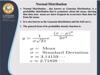
Ch 7.1 Uniform and Normal Distribution Objective B : Normal distribution Bell-shaped Curve
Example 1: Graph of a normal curve is given. Use the graph to identify the value of and . = = 530 100 2 + 2 1 1 + 530 630730X 430 330
Example 2: The lives of refrigerator are normally distributed with mean years and standard deviation years. 14 = = 5 . 2 (a) Draw a normal curve and the parameters labeled. 1 + 1 + 2 + 2 3 + 3 X 14 11 5 . 16 5 . 5 . 6 21 5 . 19 9 (b) Shade the region that represents the proportion of refrigerator that lasts for more than 17 years. 17 X 14 19 9 11 5 . 16 5 . 5 . 6 21 5 .
x (c) Suppose the area under the normal curve to the right = 17 is 0.1151. Provide two interpretations of this result. 1151 . 0 ) 17 ( = x P Notation: The area under the normal curve for any interval of values of the random variable represent either: x the proportions of the population with the characteristic described by the interval of values. 11.51% of all refrigerators are kept for at least 17 years. the probability that a randomly selected individual from the population will have the characteristic described by the interval of values. The probability that a randomly selected refrigerator will be kept for at least 17 years is 11.51%.
Ch 7.1 Uniform and Normal Distribution Objective A : Uniform Distribution Objective B : Normal distribution Ch 7.2 Applications of the Normal Distribution Objective A : Area under the Standard Normal Distribution
Ch 7.2 Applications of the Normal Distribution Objective A : Area under the Standard Normal Distribution The standard normal distribution Bell shaped curve 0 = = 1 and . = 1 = 0 5 . 3 2 5 . 3 Z 2 1 1 0 Positive Z Negative Z Z The random variable for the standard normal distribution is . Z Use the table (Table V) to find the area under the standard normal distribution. Each value in the body of the table is a cumulative area from the left up to a specific score. Z
Probability is the area under the curve over an interval. The total area under the normal curve is 1. Z Z 0 Under the standard normal distribution, = 0 5 . 0 (a) what is the area to the right of ? = 0 5 . 0 (b) what is the area to the left of ?
Example 1 : Determine the area under the standard normal curve. (a) that lies to the left of -1.38. From Table V . 0 08 . 0 0838 3 . 1 . 0 0838 . 1 0838 . 0 = ( 38 ) P Z Z . 1 0 38 From Table V . 0 (b) that lies to the right of 0.56. Table V only provides area to the left of = 0.56. 06 Z 5 . 0 . 0 7123 . 0 7123 1 Area under the whole standard normal distribution is 1. = 7123 . 0 2877 . 0 = ( . 0 56 ) 1 P Z Z 0 . 0 56
(c) that lies in between 1.85 and 2.47. 9678 . 0 From Table V . 0 47 . 2 9932 . 0 9932 . 1 85 . 0 9678 Z 9932 . 1 ( P 85 . 0 = 47 9678 . 0 . 2 ) = 0.0254 Z 0 . 2 47 . 1 85


 that lies in between 1.85 and 2.47.")