Understanding Quantum Algorithms in Data Fitting by Brian Lorn
Data fitting involves establishing relationships between data points, commonly through interpolation, extrapolation, and smoothing methods. Various types and methods of data fitting, such as linear models and statistical tests, contribute to accurate estimations and predictions in different disciplines. Implementing data fitting techniques requires statistical testing, hypothesis testing, and evaluating the strength of relationships between data.
Download Presentation

Please find below an Image/Link to download the presentation.
The content on the website is provided AS IS for your information and personal use only. It may not be sold, licensed, or shared on other websites without obtaining consent from the author. Download presentation by click this link. If you encounter any issues during the download, it is possible that the publisher has removed the file from their server.
E N D
Presentation Transcript
Quantum Algorithms in Data Fitting By Brian Lorn
Data Fitting Establish the relationship between the data points More commonly, description of how a series of independent variables contributing to a dependent variable Applications in many disciplines such as business, medical studies, scientific experiments, and many more Real observations must be written in a mathematical form Data can either be quantitative or qualitative
Types of Data Fitting Interpolation: estimating relation between known data points Estimations and predictions are limited to range of data points Extrapolation: estimating relation outside of known data points Estimations and predictions are not limited to range of data points Higher risk of uncertainty or false relationship Smoothing: creating a function that captures the most significant patterns in the data while leaving out outliers from the data Acts on the data points themselves without relying on explicit function Best at demonstrating general patterns rather than precise inferences
Methods of Data Fitting Interpolation and Extrapolation: Linear models, higher order models, interactive models, quantitative models, multiplicative models, and nested models Multivariate scale increases the complexity of the model but generally increase its accuracy as well Found through classical algorithms run through programs like R, MATLAB, and Wolfram Mathematica Smoothing: Adjacent data points are increased while individual data points that are higher or lower are reduced Linear smoothers are operations performed by a hat matrix in a process known as convolution Found through algorithms such as exponential smoothing or moving average
Implementation of Data Fitting Interpolation and Extrapolation: Statistical tests to find model adequacy Specific hypothesis testing on certain coefficients or individual variables Estimate or predict values Find the strength of the relationships between data Smoothing: Smoothed data set can be further analyzed for general patterns and other nuances Degree of error increases as data set is being modified before being analyzed
Method of Least Squares One of the most common techniques to fit data for interpolation or extrapolation Creates a best fit for the data that minimizes the sum of squared residuals in mathematical notation: In simple linear regression, the deterministic model is with Limited in only accounting for observational errors on the dependent variable Can be applied to linear, nonlinear, and higher order models Classical algorithms either use QR factorization or iteration to create a model
Method of Total Least Squares (TLS) Accounts for observational errors in both the dependent and independent variable Generalization of Deming regression (orthogonal regression) Can be applied to linear, non-linear, and higher order models In the method, the objective function is where rxand ryare vectors of residuals while Mxand Myare covariance matrices To form the model, this objective function is minimized which results in where X is the matrix of constants or functions of x and is the relationship between x and y
Classical Implementation of Method of Total Least Squares Note that SVD can be used to minimize the objective function Classical algorithms depend on the SVD for computation making the run time 26N3where N is the number of data For the partial SVD calculated through the s-step Lanczos procedure, O(N2) Difficult for classical computers to model large amounts of data
Quantum implementation of the Method of Total Least Squares TLS problem can be simplified to finding the vector vn+1which corresponds to the smallest singular value in the matrix C Obtained by solving for the eigenvectors of where C = [A, y] For simplicity, the quantum algorithm examines D = diag(C*C, . . ., C*C) Thus, the TLS problem is solved by finding the ground state of D
Quantum implementation of the Method of Total Least Squares (continued) Transition frequency between 2 energy levels of the system matches the frequency of a probe qubit Varying the frequency of the probe qubit allows the energy spectrum of the system to be determined It can then be changed to any eigenstate for any eigenvalue This can be used to compute the eigenvalues and eigenvectors matrix shown on the last slide
Quantum Algorithm and I is the identity operator, xand zare the Pauli matrices, and is the frequency of the probe qubit HRrefers to the encoded D matrix Third term is the pairing of the probe qubit and the n-qubit register of the system F transforms the reference state psi to the desired eigenstate of D
Quantum Algorithm continued In order to find the ground state of vn+1, the eigenvalue must be found The eigenvalue can be obtained by quantum simulation of resonant transitions First set range for ground eigenvalue then scan these frequency points for the probe qubit Circuit is initially set to so Then transition frequency of probe qubit is set then implement Measure probe qubit in its computational basis Repeat for all frequencies to obtain the ground state eigenvalue of the matrix D Encode this value in the Hamiltonian by setting After running the algorithm again, the probe qubit should decay to 0 kat, meaning the n-qubit register collapses to the ground state Therefore, the system evolves from its initial state to
Analysis of the Quantum Algorithm Limited by having an initial guess of the ground state D (approximate using the LS method) The runtime of the algorithm is a combination of the number of experiments that must be run to find the eigenvalue and the time needed to run each circuit The latter depends on computation cost for running the algorithm on a quantum computer Overall, the algorithm has w where k = condition number and is the precision of the guess Thus, the algorithm results in polynomial speedup
Conclusion Quantum algorithms can result in much faster computation of data fits Useful in analyzing large amounts of data that would be difficult to do with a classical algorithm Limited by the availability and complexity of Quantum computation
