Understanding Multivariate Normal Distribution and Simulation in PROC SIMNORM
Explore the concepts of multivariate normal distribution, linear combinations, subsets, and variance-covariance in statistical analysis. Learn to simulate data using PROC SIMNORM and analyze variance-covariance from existing datasets to gain insights into multivariate distributions. Visualize data through scatter plot matrices and enhance your understanding of statistical simulations.
Download Presentation

Please find below an Image/Link to download the presentation.
The content on the website is provided AS IS for your information and personal use only. It may not be sold, licensed, or shared on other websites without obtaining consent from the author. Download presentation by click this link. If you encounter any issues during the download, it is possible that the publisher has removed the file from their server.
E N D
Presentation Transcript
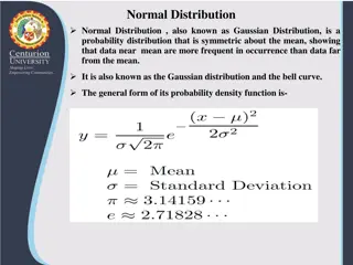
The Normal Distribution 2 1 2 x 1 = = pdf ( ) f x e 2 a = = cdf ( ) a ( ) f x dx = = Mea Variance n ( ) ([ E X = = 2 2 ] ) E x We write : ( , ) x N 2
The Multivariate Normal x x 1 1 11 12 1 k 2 2 21 22 2 k = = = x x 1 2 k k k k kk 1 k 1 2 = 1 ( ) x x { ( ) ( )} f exp x 1 (2 ) | | 2 2 Defines the multivariate normal with mean and variance-covariance matrix , denoted MVN( , ) x 3
Subsets of a MVN are also MVN with mean gotten by taking the correct elements from and variance and variance gotten by taking the correct rows and columns from 4
Linear Combinations of MVNs are also MVNs If ~ x ( , ) MVN = Y AX and ' Y A A A Then ~ ( , ) MVN 5
Simulation with PROC SIMNORM %let obs = 1000; %let seed=54321; /* create a TYPE=COV data set */ data data ACov(type=COV); input _TYPE_ $ 1 1-8 8 _NAME_ $ 9 9-16 datalines; COV x1 3 2 1 COV x2 2 4 0 COV x3 1 0 5 MEAN 1 2 3 run run; proc proc simnormal simnormal data=ACov outsim=MVN nr = &obs /* size of sample */ seed = &seed; /* random number seed */ var x1-x3; run run; 16 x1 x2 x3; 7
Create scatter plot matrix of simulated data proc proc corr plots(maxpoints=NONE)=matrix(histogram); var x:; run run; corr data=MVN COV 8
Variance-covariance from existing Data %let vars=age bmi sbp dbp; proc proc corr noprint; var &vars; run run; proc proc contents contents data=cov1;run proc proc print print data=cov1; run run; corr data=fram.frex4 outp=cov1 cov run; 10
Read type=corr dataset in IML proc proc iml use cov1; read all var _num_ where(_TYPE_="COV") into cov[r=_NAME_ c=VarNames]; read all var _num_ where(_TYPE_="CORR") into corr; read all var _num_ where(_TYPE_="MEAN") into mean; read all var _num_ where(_TYPE_="STD" ) into std; close cov1; print cov, mean, std, corr; quit quit; iml; 11
Simulate using Proc SimNorm %let n = 1000; %let seed=54321; proc proc simnormal simnormal data=Cov1 outsim=MVN nr = &n seed = &seed; var &vars; run run; proc proc corr plots(maxpoints=NONE)=matrix(histogram); var &vars; run run; corr data=MVN COV 12
Converting Between Correlation and Covariance Matrices 1 1 0 0 0 0 11 11 11 12 13 11 12 13 = 0 0 0 0 21 22 23 22 21 22 23 22 0 0 0 0 31 32 33 31 32 3 3 33 33 13
Converting Between Correlation and Covariance Matrices proc iml iml; /*convert covariance to correlation example matrix from sas help*/ S = {1.0 1.0 1.0 1.0 8.1 8.1, 1.0 1.0 16.0 16.0 18.0 18.0, 8.1 8.1 18.0 18.0 81.0 81.0 }; print s; D = sqrt(diag(S)); print d; r=inv(d)*s*inv(d); print r; cov=d*r*d; print s,cov; /*SAS functions in the IMLMLIB library cov2corr corr2cov*/ corr=cov2corr(s); print corr; cov1=corr2cov(r,vecdiag(d)); print cov1; quit quit; proc 14
When is a correlation matrix not a correlation matrix? proc proc iml /*a correlation*/ d = {1.0 1.0 0.3 0.3 0.3 1.0 0.6 0.6 0.6 eigval_d = eigval(d); print d,eigval_d; /*not a correlation*/ C = {1.0 1.0 0.3 0.3 0.9 0.3 0.3 1.0 1.0 0.9 0.9 0.9 0.9 0.9 1.0 eigval_c = eigval(C); print c,eigval_c; quit quit; iml; 0.3 0.6 1.0 0.6 0.6 1.0 0.6, 0.6, 1.0}; 0.9, 0.9, 1.0}; 15
Checking whether a matrix is symetric and positive definite A = { 2 2 -1 1 0 0, -1 1 2 2 -1 1, 0 0 -1 1 2 2 }; proc proc iml iml; /* finite-precision test of whether a matrix is symmetric */ start SymCheck(A); B = (A + A`)/2 2; scale = max(abs(A)); delta = scale * constant("SQRTMACEPS"); return( all( abs(B-A)< delta ) ); finish; /* test a matrix for symmetry */ IsSym = SymCheck(A); print IsSym; /*check for positive semi-definite using root*/ G = root(A, "NoError"); if G=. . then print "The matrix is not positive semidefinite"; /* check for positive-definite using eigval function*/ eigval = eigval(A); print eigval; if any(eigval<0 0) then print "The matrix is not positive semidefinite"; else if all(eigval>0 0) then print "Matrix is positive-definite"; else print "Matrix is Positive Semi-definite"; quit quit; 16
