Understanding Heteroskedasticity in Regression Analysis
Learn about the impact of heteroskedasticity on OLS estimations in regression analysis, including causes, consequences, and detection methods. Explore how violations of classical assumptions can affect the validity of inferences made in econometrics.

Download Presentation

Please find below an Image/Link to download the presentation.
The content on the website is provided AS IS for your information and personal use only. It may not be sold, licensed, or shared on other websites without obtaining consent from the author. If you encounter any issues during the download, it is possible that the publisher has removed the file from their server.
You are allowed to download the files provided on this website for personal or commercial use, subject to the condition that they are used lawfully. All files are the property of their respective owners.
The content on the website is provided AS IS for your information and personal use only. It may not be sold, licensed, or shared on other websites without obtaining consent from the author.
E N D
Presentation Transcript
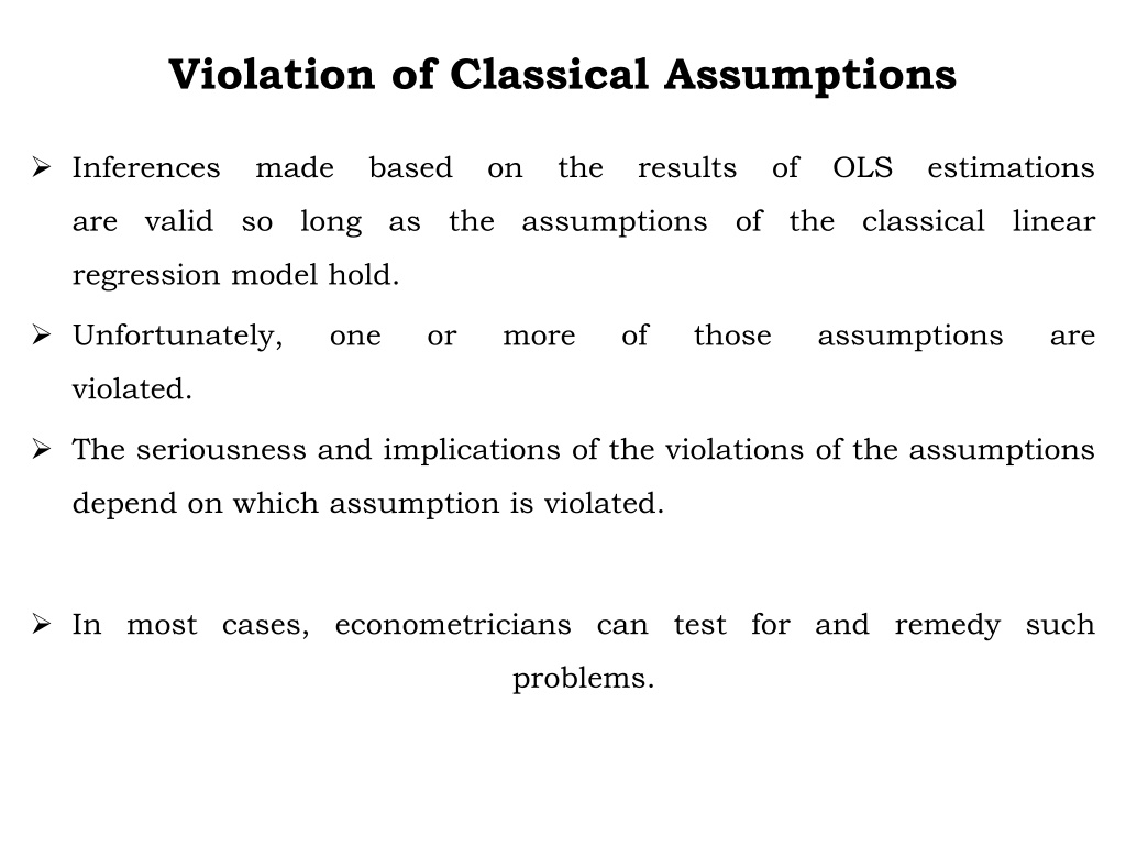
Violation of Classical Assumptions Inferences made based on the results of OLS estimations are valid so long as the assumptions of the classical linear regression model hold. Unfortunately, one or more of those assumptions are violated. The seriousness and implications of the violations of the assumptions depend on which assumption is violated. In most cases, econometricians can test for and remedy such problems.
Heteroskedasticity The homoskedasticity assumption states that the variance of the unobservable error /explanatory variables, is constant. Homoskedasticity is needed to justify the usual t tests, F tests, and confidence intervals for OLS estimation of the linear regression model, even with large sample sizes. Homoskedasticity fails whenever the variance u, conditional on the of the unobservables changes across different segments of the population, which are determined by the different values of the explanatory variables. For example, regressing typing skills against time
Hetro. Heteroskedasticity tends to occur when the variance of the unobservable across different segments of the population with the explanatory variables. changes Under heteroskedasticity, the OLS estimates of s s are still unbiased, and consistent. Moreover, the interpretation of the R2 and adjusted R2 is is heteroskedasticity. not affected under
Hetro. Cause of Heteroschedasity: Error learning model Improvement in data collection technique Presence of outliers
Hetro. consequences of heteroskedasticity for ols: Unbiased estimators Biased variance and they are no longer valid for constructing confidence intervals and t statistics. Inefficient estimators the usual OLS t statistics do not have t distributions in the presence of heteroskedasticity, similarly, F statistics are no longer F distributed, thus, the statistics we used to test hypotheses are not valid in the presence of heteroskedasticity. OLS is no longer BLUE
Detecting Heteroskedasticity It may be generally the rule instead of expectation to face heteroskedasticity in cross sectional data. The graph of the square of the residual against the dependent variable gives rough indication of the existence of of heteroskedasticity. If there appears a systematic trend in the graph it may be an indication of the existence of heteroskedasticity. There are however formal methods of detecting heteroskedasticy.
Hetro. The Breusch-Pagan Test Given the regression equation: ?0+ ?1?1+ ?2?2+ + ????+ ?? 1 the Breusch-Pagan test for heteroskedasticity is carried out as follows: 1. Estimate the Equation 1 by OLS and obtain the residual. 1. run the regression: ?2= ?0+ ?1?1+ ?2?2+ ????+ ?? and obtain R squared for the residual ? ?2? 2. Form the F-statistic: ? = 1 ? ?2 ? ? 1 A small p-value rejects the null of homoskedasticity.
Hetro. The White s General HeteroskedasticityTest Given the regression model under equation 1 the white s test for k = 3 proceeds as follows. 1. 2. Run regression on equation 1 with k = 3 and obtain ?2. Run the auxiliary regression: ?2= ?0+ ?1?1+ ?2?2+ ?3?3+ ?4?12+ ?5?22 rationale of including the independent variables, their squares, and cross products is that the variance may be systematically correlated with either of the independent variables linearly or non-linearly + ?6?32+ ?? The The null is that:?1= ?2= ?3= ?4= ?5= ?6= 0 Obtain R2 from the regression Then: If we fail to reject the null, we conclude that there is homoskedasticity
Hetero. Dealing with Heteroscedasticity In the last two decades, econometricians have learned how to adjust standard errors, so that t, F, and LM statistics are valid in the presence of heteroskedasticity. This is very convenient because it means we can report new statistics that work, regardless of the kind of heteroskedasticity population. present in the
Hetero. While heteroscedasticity is the property of disturbances, the above tests deal with residuals. Thus, they may not report the genuine heteroskedasticity. Diagnostic results against homoskedasticity could be due to misspecification of the model. But, if we are sure that there is a genuine heteroskedasticity problem, we can deal with the problem using: Heteroskedasticity-robust statistics after estimation by OLS. Weighted least squares (WLS) estimation.
Autocorrelation It occurs when the classical assumption that:??? ??,?? = 0 ??? ? ? ?? ????????. It occurs most frequently when estimating models using time series data, and, hence also called serial correlation. The most popular way of modeling serially correlated disturbances has been to replace the classical assumptions concerning tby: ??= ??? 1+ ?? where is a parameter such that 1 1, and is error term with CLRM assumptions holding. It is called a first order autoregressive (AR) process.