Understanding Frequency, Stem-and-Leaf Graphs, and Histograms in Data Analysis

Frequency, relative frequency, and cumulative relative frequency are explained with examples. Stem-and-leaf graphs help in organizing small data sets, while histograms display data with continuous variables. An example with heights of male soccer players demonstrates constructing histograms. Calculating bar widths is also discussed.

Download Presentation

Please find below an Image/Link to download the presentation.
The content on the website is provided AS IS for your information and personal use only. It may not be sold, licensed, or shared on other websites without obtaining consent from the author. Download presentation by click this link. If you encounter any issues during the download, it is possible that the publisher has removed the file from their server.
E N D
Presentation Transcript
Lecture Notes Frequency, Stem-and-Leaf Graphs , Histograms Prof. Xin, Ke OER www.helpyourmath.com
Frequency A frequency is the number of times a value of the data occurs. A relative frequency is the ratio (fraction or proportion) of the number of times a value of the data occurs in the set of all outcomes to the total number of outcomes. Cumulative relative frequency is the accumulation of the previous relative frequencies. Example: 5; 6; 3; 3; 2; 4; 7; 5; 2; 3; 5; 6; 5; 4; 4; 3; 5; 2; 5; 3. Data value Frequency RELATIVE FREQUENCY CUMULATIVE RELATIVE FREQUENCY 0.15 0.15+0.25=0.40 0.40+0.15=0.55 0.55+0.30=0.85 0.85+0.10=0.95 0.95+0.05=1.00 2 3 4 5 6 7 3 5 3 6 2 1 3/20=0.15 5/20=0.25 3/20=0.15 6/20=0.30 2/20=0.10 1/20=0.05
Stem-and-Leaf Graphs (Stemplots) stem-and-leaf graph or stemplot, comes from the field of exploratory data analysis. It is a good choice when the data sets are small. To create the plot, divide each observation of data into a stem and a leaf. The leaf consists of a final significant digit. Example: 33; 42; 49; 49; 53; 55; 55; 61; 63; 67; 68; 68; 69; 69; 72; 73; 74; 78; 80; 83; 88; 88; 88; 90; 92; 94; 94; 94; 94; 96; 100 Stem Leaf 3 3 4 2 9 9 5 3 5 5 6 1 3 7 8 8 9 9 7 2 3 4 8 8 0 3 8 8 8 9 0 2 4 4 4 4 6 10 0
Histograms A histogram consists of contiguous (adjoining) boxes. It has both a horizontal axis and a vertical axis. The horizontal axis is labeled with what the data represents. The vertical axis is labeled either frequency or relative frequency. To construct a histogram, first decide how many bars or intervals, also called classes, represent the data. Many histograms consist of five to 15 bars or classes for clarity. The number of bars needs to be chosen. Choose a starting point for the first interval to be less than the smallest data value. A convenient starting point is a lower value carried out to one more decimal place than the value with the most decimal places. (For example, if the value with the most decimal places is 6.1 and this is the smallest value, a convenient starting point is 6.05(6.1 0.05=6.05).)
Histograms Example The following data are the heights (in inches to the nearest half inch) of 100 male semiprofessional soccer players. The heights are continuous data, since height is measured. 60; 60; 61; 61; 61; 63; 63; 63; 64; 64; 64; 64; 64; 64; 64; 64; 64; 64; 64; 64; 64; 64; 64; 66; 66; 66; 66; 66; 66; 66; 66; 66; 66; 66; 66; 66; 66; 66; 66; 66; 66; 66; 66; 66; 67; 67; 67; 67; 67; 67; 67; 67; 67; 67; 67; 67; 67; 67; 67; 67; 67; 67; 67 68; 68; 69; 69; 69; 69; 69; 69; 69; 69; 69; 69; 69; 69; 69; 69; 69 70; 70; 70; 70; 70; 70; 70; 70; 70; 71; 71; 71 72; 72; 72; 72; 72; 73; 73; 74
Width Next, calculate the width of each bar or class interval. To calculate this width, subtract the starting point from the ending value and divide by the number of bars (you must choose the number of bars you desire). width of a class = ??????? ????? ?? ???? ??? ?????? ????? ?? ???? ??? choose an integer for width value. Therefore, we choose the number s integer part and plus 1 as width. We get . However, we will ??????? ?????? ?? ????? Classes 60 ~ 61 62 ~ 63 64 ~ 65 66 ~ 67 68 ~ 69 70 ~ 71 72 ~ 73 74 ~ 75 width of a class =[??????? ????? ?? ???? ??? ?????? ????? ?? ???? ??? ??????? ?????? ?? ????? ] + 1 In the example, the highest value in data set is 74, the lowest value in data set is 60. We can desire number of class is 8, so we can get: Width of a class = 74 60 integer part and plus 1 as width. Therefore, width = [1.75]+1=2 = 1.75, but we will choose the number s 8 Then, we can get the classes on the right side:
The class has class limits, and they are lower class limits(LCL) and upper class limits(UCL). The class boundary also has lower class boundary(LCB) and upper class boundary(UCB). The relationship between class and boundary: LCB=LCL -? where D is the difference between the LCL of the next class interval and the UCL of the given class interval. ?and UCB=UCL + ? (1) ? boundaries 59.5 ~ 61.5 61.5 ~ 63.5 63.5 ~ 65.5 65.5 ~ 67.5 67.5 ~ 69.5 69.5 ~ 71.5 71.5 ~ 73.5 73.5 ~ 75.5 From above, we still can get: LCL=LCB + ? ?and UCL=UCB -? (2) ? In the example: D = LCL - LCB = 61 60 = 0.5 2 Therefore, we can get the boundaries on the right side:
Table: Scores on a midterm exam Cumulative Frequency Classes Class Boundaries Frequency Midpoint Relative Frequency 5 (60+61)/2=60.5 5/100=0.05 0.05 60 ~ 61 62 ~ 63 64 ~ 65 66 ~ 67 68 ~ 69 70 ~ 71 72 ~ 73 74 ~ 75 59.5 ~ 61.5 61.5 ~ 63.5 63.5 ~ 65.5 65.5 ~ 67.5 67.5 ~ 69.5 69.5 ~ 71.5 71.5 ~ 73.5 73.5 ~ 75.5 3 (62+63)/2=62.5 3/100=0.03 0.05+0.03=0.08 15 (64+65)/2=64.5 15/100=0.15 0.08+0.15=0.23 40 (66+67)/2=66.5 40/100=0.4 0.23+0.4=0.63 17 (68+69)/2=68.5 17/100=0.17 0.63+0.17=0.8 12 (70+71)/2=70.5 12/100=0.12 0.8+0.12=0.92 7 (72+73)/2=72.5 7/100=0.07 0.92+0.07=0.99 1 (74+75)/2=74.5 1/100=0.01 0.99+0.01=1
The following histogram displays the heights on the x-axis and relative frequency on the y-axis. Heights
Practice 1 For data set below, create a histogram with 6 classes. 76,84,76,103,92, 47,98,54,80,91, 69,86,83,75,93 69,86,83,75,93 89,96,65,94,85 Solution Video
Practice 2 For data set below, create a histogram with 6 classes. 4.53,3.83,3.83,4.23,4.70, 1.83,4.00,2.00,3.57,4.25, 2.75,4.47,3.35,3.27,4.30, 4.25,4.05,2.12,4.63,4.18, Solution Video


")