Bayesian Classification and Intelligent Information Retrieval
Bayesian classification involves methods based on probability theory, with Bayes' theorem playing a critical role in probabilistic learning and categorization. It utilizes prior and posterior probability distributions to determine category given a description. Intelligent Information Retrieval complements this by utilizing conditional probability and independence for effective categorization. The process involves estimating priors and conditionals from data to classify instances accurately.
Download Presentation

Please find below an Image/Link to download the presentation.
The content on the website is provided AS IS for your information and personal use only. It may not be sold, licensed, or shared on other websites without obtaining consent from the author. Download presentation by click this link. If you encounter any issues during the download, it is possible that the publisher has removed the file from their server.
E N D
Presentation Transcript
Text/Document Categorization Part II Bayesian Classification CSC 575 Intelligent Information Retrieval
Bayesian Methods for Classification Learning and classification methods based on probability theory. Bayes theorem plays a critical role in probabilistic learning and classification. Uses prior probability of each category given no information about an item. Categorization produces a posterior probability distribution over the possible categories given a description of an item. 2 Intelligent Information Retrieval
Conditional Probability & Independence P(A | B) is the probability of A given B Assumes that B is all and only information known. Note that in general: ) ( B A P = ( | ). ( ) P A B P B But, if A and B are independent, then = = ( | ) ( ) P A B P A ( | ) ( ) P B A P B = and so: ( ) ( ) ( ) P A B P A P B 3 Intelligent Information Retrieval
Bayess Rule Let s again consider the definition: = ( ) ( | ). ( ) P A B P A B P B = ( ) ( | ). ( ) P A B P A B P B Bayes s Rule: Direct corollary of above definition = ( ) ( | P = ). B ( ) P B A P B = A P A but P ( ) ( ) A P A B A ( | ). ( ) ( | ). ( ) A B P B P B P A ( | P ). B ( ) P B A P A = ( | ) P A B ( ) ( | P ) ( ) P E H P H Often written in terms of hypothesis and evidence: = ( | ) P H E ( ) E 4
Bayesian Categorization Letset of categories be {c1, c2, cn} Let E be description of an instance Determine category of E by determining for each ci ( ) P ( E | ) P c P E c = ( | ) i i P c E i ( ) P(E) can be determined since categories are complete and disjoint. ( ) ( | ) n n P c P ( E ) c = i = i = = ( | ) 1 i i P c E i P E 1 1 n = i = ( ) ( ) ( | ) P E P c P E c i i 1 5 Intelligent Information Retrieval
Bayesian Categorization (cont.) Need to know: Priors: P(ci) Conditionals: P(E | ci) ( ) P ( E | ) P c P E c = ( | ) i i P c E i ( ) P(ci) are easily estimated from data. If ni of the examples in D are in ci,then P(ci) = ni / |D| For we need to consider the feature representation of the instance E to be classified: ? = ?1,?2, ,?? 6 Intelligent Information Retrieval
Nave Bayesian Categorization ? = ?1,?2, ,?? Too many possible instances (exponential in m) to estimate all P(E | ci) But, if we assume features of instance E are conditionally independent given the category (ci), then ? ?(?|??) = ?(?1,?2, ,??|??) = ?(??|??) ?=1 Therefore, we then only need to know P(ej | ci) for each feature and category. 7 Intelligent Information Retrieval
Nave Bayes Example C = {allergy, cold, well} e1 = sneeze; e2 = cough; e3 = fever E = {sneeze, cough, fever} Prob Well Cold Allergy P(ci) 0.9 0.05 0.05 P(sneeze|ci) P(cough|ci) P(fever|ci) 0.1 0.9 0.9 0.1 0.8 0.7 0.01 0.7 0.4 8 Intelligent Information Retrieval
Nave Bayes Example (cont.) Probability Well Cold Allergy P(ci) P(sneeze | ci) P(cough | ci) P(fever | ci) 0.9 0.05 0.05 0.1 0.9 0.9 E={sneeze, cough, fever} 0.1 0.8 0.7 0.01 0.7 0.4 P(well | E) = P(well) P(E | well) / P(E) But, P(E | well) = P(sneeze | well)*P(cough | well)*(1- P(fever | well) = (0.1)(0.1)(0.99) And, P(well) = 0.9 So: P(well | E) = (0.9)(0.1)(0.1)(0.99)/P(E)=0.0089/P(E) Similarly, we must compute P(Cold |E) and P(Allergy | E) 9 Intelligent Information Retrieval
Nave Bayes Example (cont.) Probability Well Cold Allergy P(ci) P(sneeze | ci) P(cough | ci) P(fever | ci) 0.9 0.05 0.05 0.1 0.9 0.9 E={sneeze, cough, fever} 0.1 0.8 0.7 0.01 0.7 0.4 P(well | E) = (0.9)(0.1)(0.1)(0.99)/P(E)=0.0089/P(E) P(cold | E) = (0.05)(0.9)(0.8)(0.3)/P(E)=0.01/P(E) P(allergy | E) = (0.05)(0.9)(0.7)(0.6)/P(E)=0.019/P(E) Now we can obtain P(E): P(E) = 0.089 + 0.01 + 0.019 = 0.0379 P(well | E) = 0.24 P(cold | E) = 0.26 P(allergy | E) = 0.50 10 Intelligent Information Retrieval
Estimating Probabilities Normally, probabilities are estimated based on observed frequencies in the training data. If D contains niexamples in class ci, and nij of these ni examples contains feature/attribute ej, then: n ij = ( | ) P e c j i n i If the feature is continuous-valued, P(ej|ci) is usually computed based on Gaussian distribution with a mean and standard deviation 2 ( ) x 1 = 2 ( , , ) g x e 2 2 and P(ej|ci) is = ( | ) ( , , ) P e g e ci j j c c i i 11
Smoothing Estimating probabilities from small training sets is error-prone: If due only to chance, a rare feature, ek, is always false in the training data, ci :P(ek | ci) = 0. If ek then occurs in a test example, E, the result is that ci: P(E | ci) = 0 and ci: P(ci | E) = 0 To account for estimation from small samples, probability estimates are adjusted or smoothed Laplace smoothing using an m-estimate assumes that each feature is given a prior probability, p, that is assumed to have been previously observed in a virtual sample of size m. + n mp ij = ( | ) P e c j i + n m i For binary features, p is simply assumed to be 0.5. 12
Nave Bayes Classification for Text Modeled as generating a bag of words for a document in a given category by repeatedly sampling with replacement from a vocabulary V = {w1, w2, wm} based on the probabilities P(wj| ci). Smooth probability estimates with Laplace m-estimates assuming a uniform distribution over all words p = 1/|V|) and m = |V| Equivalent to a virtual sample of seeing each word in each category exactly once. 13 Intelligent Information Retrieval
Text Nave Bayes Algorithm (Train) Let V be the vocabulary of all words in the documents in D For each category ci C Let Dibe the subset of documents in D in category ci P(ci) = |Di| / |D| Let Ti be the concatenation of all the documents in Di Let ni be the total number of word occurrences in Ti For each word wj V Let nij be the number of occurrences of wj in Ti Let P(wi| ci) = (nij + 1) / (ni + |V|) 14 Intelligent Information Retrieval
Text Nave Bayes Algorithm (Test) Given a test document X Let n be the number of word occurrences in X Return the category: n = max ( ) c C i ( | ) P c P a c i i i 1 i where ai is the word occurring the ith position in X Alternative (log-based) approach to avoid underflow to very small probability values (take the log, resulting in a sum of logs): ? ? max ?? ? log ? ?? ?=1 + ?=1 ?(??|?? ] = max log ? ?? log(? ????)) ?? ? 15 Intelligent Information Retrieval
Text Nave Bayes Example 1 Doc 1 2 3 4 5 Words Chinese Beijing Chinese Chinese Chinese Shanghai Chinese Macao Tokyo Japan Chinese Chinese Chinese Chinese Tokyo Japan Class c c c j ? P(c)=Nc Training N P(w|c)=count(w,c)+1 count(c)+|V | Test Choosing a class: P(c|d5) Priors: P(c) = 3/4 P(j) = 1/4 3/4 * (3/7)3 * 1/14 * 1/14 0.0003 Conditional Probabilities: P(Chinese|c) = (5+1) / (8+6) = 3/7 P(Tokyo|c) = (0+1) / (8+6) = 1/14 P(Japan|c) = (0+1) / (8+6) = 1/14 P(Chinese|j) = (1+1) / (3+6) = 2/9 P(Tokyo|j) = (1+1) / (3+6) = 2/9 P(Japan|j) = (1+1) / (3+6) = 2/9 P(j|d5) 1/4 * (2/9)3 * 2/9 * 2/9 1/4 * (2/9)3 * 2/9 * 2/9 0.0001 0.0001 Can obtain actual probabilities via normalization (though, not needed for classification): P(c|d5) P(j|d5) = 0.0001/(0.0003+0.0001) = 75% = 0.0003/(0.0003+0.0001) = 25%
Nave Bayes Example 2: Spam Filtering t1 2 0 0 1 0 1 0 0 0 4 t2 1 0 3 2 1 1 1 1 0 2 t3 0 1 1 0 2 0 0 4 1 0 t4 3 1 0 1 1 0 0 1 1 0 t5 0 0 1 2 0 1 1 0 2 1 Spam no no yes yes yes no yes yes no yes P(no) = 0.4 P(yes) = 0.6 Priors: D1 D2 D3 D4 D5 D6 D7 D8 D9 D10 P(w|c)=count(w,c)+1 count(c)+|V | Training Data Total word occurrences for no + |V| = 15 + 5 = 20 Total word occurrences for yes + |V| = 30 + 5 = 35 Cond. Probabilities: Term t1 t2 t3 t4 t5 P(t|no) 4/20 3/20 3/20 6/20 4/20 P(t|yes) 6/35 11/35 8/35 4/35 6/35 E.g., P(t1|no) = [(2+0+1+0) +1] / 20 = 4/20 Now consider a New email x containing t1, t4, t5, t4, t4, t2, t5, t4 Need to find P(yes | x) and P(no | x) Should it be classified as spam = yes or spam = no ?
Text Nave Bayes - Example Cond. Probabilities: Priors: New email x: t1, t4, t5, t4, t4, t2, t5, t4 Term t1 t2 t3 t4 t5 P(t|no) 4/20 3/20 3/20 6/20 4/20 P(t|yes) 6/35 11/35 8/35 4/35 6/35 P(no) = 0.4 P(yes) = 0.6 i.e., the vector: [1, 1, 0, 4, 2] P(yes | x) = [6/35 * 11/35 * (4/35)4 * (6/35)2] * P(yes) / P(x) = 2.70e-07 * 0.6/ P(x) = 0.000000162 / P(x) P(no | x) = [4/20 * 3/20 * (6/20)4 * (4/20)2] * P(no) / P(x) = 0.00000972 * 0.4 / P(x) = 0.00000389 / P(x) P(no | x) = 0.00000389 / (0.000000162 + 0.00000389) = 0.96 P(yes | x) = 0.000000162 / (0.000000162 + 0.00000389) = 0.04 Note that we don t actually need to compute complete probabilities (so, we don t need to use normalization to compute p(x) in the denominators) because we are only interested in the relative probabilities. In this case, clearly the probability P(no | x) will be much higher than P(yes |x) based on the two numerators in above expressions. To avoid underflow in cases of very small numbers, we could instead use the sum of logs method, e.g., P(yes | x) [ Log(6/35) + Log(11/35) + Log(4/35)*4 + Log(6/35)*2 ] + LOG(6/10) = -6.79
Text/Document Categorization CSC 575 Intelligent Information Retrieval
