Understanding Challenges Faced by the Near-Poor and Strategies for Development
The analysis explores the concept of the near-poor, highlighting socioeconomic challenges they face due to being excluded from social assistance despite living precarious lives. It questions the government's stance, considering budget constraints and urgent needs of the poor. The discussion extends to operational definitions, strategy development, and ways to support the near-poor without compromising poverty alleviation efforts.
- Near-Poor Challenges
- Socioeconomic Inclusiveness
- Government Strategy
- Poverty Thresholds
- Social Assistance
Download Presentation

Please find below an Image/Link to download the presentation.
The content on the website is provided AS IS for your information and personal use only. It may not be sold, licensed, or shared on other websites without obtaining consent from the author. Download presentation by click this link. If you encounter any issues during the download, it is possible that the publisher has removed the file from their server.
E N D
Presentation Transcript
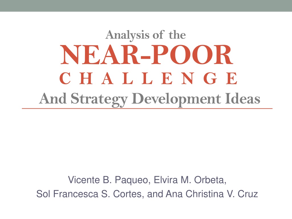
Analysis of the NEAR-POOR C H A L L E N G E And Strategy Development Ideas Vicente B. Paqueo, Elvira M. Orbeta, Sol Francesca S. Cortes, and Ana Christina V. Cruz
Context 1: CONCERN ABOUT CYCLICAL POVERTY households (HH) moving in and out of poverty is quite high Persistent poor Persistent Non-Poor Transients % of 8.9 38.6 52.45 households APIS Panel Data 2004-2010 Persistent poor (non-poor) are households with income less (greater) than official total poverty threshold (TPT) in all APIS survey years during 2004-2010. Transients are households whose income is less than TPT at least once during the same period.
Contextt 2: CONCERN ABOUT STINGINESS of the total poverty threshold (TPT) Households above the official TPT at a given year are classified as non-poor due to the stinginess of the TPT They are, therefore, officially excluded from social assistance like the Pantawid Pamilya In reality, many of them live difficult and precarious lives with high risk of becoming poor any time soon These non-poor HHs called the near-poor in the literature is increasingly becoming a concern in the light of the inclusiveness goal
QUESTIONS: Operationally, who are the Near-Poor? What are the socioeconomic challenges they are facing? What should be the stance of the Government, given its budget constraints and the more urgent needs of the poor? What (if any) can the Government do to meet the challenges of the near-poor without undermining its ability to help get them out of poverty? What can the near-poor do on their part?
Structure of presentation Part 1: The near-poor: concept, practical estimation methods and profile - Part 2: Rationing of Social Assistance When Budget Is Insufficient to Cover All the Near-Poor Households - Part 3: Near-poor strategy development
Definitions of Near-Poor in the Literature Poverty Threshold Measure Used Definition of Near-poor Reference three times the cost of minimum food diet in 1963 Orshansky (1966); Individuals with family income between 100 and 133 percent of the official poverty threshold Heggeness and Hokayem (2013) three times the cost of minimum food diet in 1963 Hokayem and Heggeness (2014) Individuals with family income between 100 and 125 percent of the poverty thresholds National Academy of Sciences (NAS) measure Ben-Shalom, Moffitt and Scholz (2011) Those living between 100 and 150 percent of poverty Supplemental Poverty Measure (SPM) Short and Smeeding (2012) Those with modest incomes - living between 100 to 200 percent of poverty US$1.25 a day (@2005 PPP) absolute poverty line ILO (2013) Workers with per-capita household consumption of between US$2.0 to US$4.0 a day ( i.e., between 160 to 220 percent of poverty) US$2.0 a day 2009 official poverty line Chua (2013) Vulnerable non-poor those whose income is within 20% above the poverty line US$1.20 a day 2011 national poverty line in Indonesia Jellema and Noura (2012) Those with consumption of approximately 1.2x the poverty line lowest three deciles Harimurti et al. (2013) Lowest three deciles based on household consumption as covered by the Indonesian health insurance program intended for the poor and near- poor Table 6. on study
Part 1 THE NEAR-POOR: Concept, Practical Estimation Methods And Profile
Finding: Ratio (RAT) of Near-Poverty Threshold (NPT) to Total Poverty Threshold (TPT) Clusters Around 1.1- 1.37 NPT-TPT ratio (RAT) % above TPT 10 20 25 25 PhilHealth World Bank Vietnam US Census Bureau (Hokayem and Heggeness, 2014) Orshansky (pre-2014) 1.1 1.2 1.25 1.25 1.33 33 28 37 1.28 (knife-edge) 1.37 (balik-balik) Authors Estimate
NPT Amount (in 2014 Pesos) by Different RAT Levels: % over TPT 27, 596 37% = Authors (Balik-Balik) 26, 790 33% = Orshansky Amount equivalent in Php 28% = Authors(Knife-Edge) 25, 783 24, 179 25% = Vietnam; US Census 24, 172 20% = World Bank 22,157 10% = PhilHealth 20,143 Annual Per Capita Poverty Threshold
Comments on Previous RATs Based on income distribution of households NOT considering the risk of subsequent poverty How did we estimate our RATs?
Methodology for the Balik-Balik RAT estimate of 1.37 We define the Balik-Balik (cyclical) poor as households who move in and out of poverty during a given time period between 2004-2010 (also called transients). We consider the mean household income of the transients (MINC) as the NPT for the Balik-Balik households. The Balik-Balik RAT = MINC/TPT = 1.37
Methodology for Knife-Edge RAT Estimate of 1.28 We use the following working definition - Per capita income above the official total poverty threshold (TPT) at a given year, but at high risk of subsequently falling into poverty soon - Metaphorically, non-poor households that precariously live at a knife-edge with little or no buffer against the economic effects of idiosyncratic and covariate shocks The NPT is chosen at the level of household income that implies a risk of subsequent poverty of at least 50%
Methodology for Knife-Edge RAT Estimate of 1.28 RSKj = a + b (1/PCY) for j = e, d where RSKe= mean number of poverty episodes in 2007-2010 experienced by the non-poor households of 2004, as a percent of number of survey years RSKd = percent of non-poor households in 2004 becoming poor at least once in 2007-2010 PCY = per capita household income
Regression equation estimates relating poverty risk of non-poor households to income RSKd -.2326382 RSKe -.189562 Constant (-4.43) (-5.27) 1/Per Capita income 9083.147 (12.69) 5663.6 (11.56) Adjusted R-squared (goodness of it measure) 0.9468 0.9365 Number of Observations = 10 (mean values of 10 inome classes)
Predicted Poverty Risk (RSKj) of Non-Poor Households, Using NHTS-PR Proxy Means Test Income Estimates Frequency distribution of non- poorc 14% 12% 11% 9% 8% 6% 5% 5% 4% 3% 23% NPT =Mean income per capitaa RAT = NPT/TPTb Predictedd RSKd Predictedd RSKe 1.05 1.15 1.25 1.35 1.45 1.55 1.65 1.75 1.85 1.95 2.82 66% 58% 52% 46% 41% 37% 34% 30% 27% 25% 10% 37% 32% 28% 24% 21% 19% 17% 15% 13% 11% 2% 10,163 11,129 12,095 13,072 14,039 15,004 15,968 16,921 17,905 18,872 27,310
Checking out the exclusion and inclusion error rates RAT Exclusion Error Rate 1.1 (PhilHealth) 36% 1.2 (World Bank) 20% 1.28 (Knife-edge) 12% 1.37 (Balik-balik) 8% Exclusion Error those with HIGH risk of subsequently falling into poverty but excluded because of income greater than NPT. Inclusion Error those with LOW risk of subsequently falling into poverty but included because income less than NPT . Inclusion Error Rate 2% 4% 7% 11%
Use of RAT is a good practical approach, particularly when panel data are not available to link NPT to RSK Inclusion error rate is minimal (only 2 percent) at RAT 1.10 and rises moderately to just 7 percent at RAT 1.28 or to 11 percent at RAT 1.37 Exclusion error rate is a high of 36 percent at RAT 1.10 but falls to a moderate rate of 12 percent at RAT 1.28 or to a lower rate of 8 percent at 1.37 Memo: The choice of low RAT due for example to tight budget would probably lead to a great number of high risk, near-poor households
Exclusion/ inclusion errors are MANAGABLE. Two ways of managing the errors Increase RAT, as additional budget becomes available to reduce the exclusion error rates without unduly raising inclusion errors Prioritize high risk near-poor households (methodology in Part 2)
Mean Characteristics of Near-Poor (RAT= 1.28) (a) Income and Expenditures Closer to Poor (b) Savings are positive for the near-poor but negative for the poor 2010 Near-Poor Profiles All HHs Poor Non Poor Distribution (%) 100 22.93 12.15 64.93 Total Income1 106,385 41,090 57,593 138,567 Wages and Salaries 1 42,900 14,435 22,842 56,703 Entrepreneurial Income1 29,282 15,583 20,566 35,749 Total Expenditures1 94,250 43,751 56,352 119,170 Education Expenditures1 4,715 971 1,639 6,613 Medical Expenditures1 3,060 462 948 4,373 Savings2 12,135 -2,661 1,240 19,397 Notes 1/ The household mean income and expenditure values are in pesos expressed in 2000 prices. 2/ Savings = Total Income Total Expenditure
Mean characteristics of the near-poor: more human and physical assets 2010 Near- Poor Profiles All HHs Poor Non Poor Education, assets and location % Did not graduate high school % Own Lot % with Own Electricity % with Own Water % Houses made of Strong/Predominantly Strong Materials % Urban Household Notes 1/ The household mean income and expenditure values are in pesos expressed in 2000 prices. 2/ Savings = Total Income Total Expenditure 59.4 83.28 75.5 47.95 74.4 86.12 38.76 66.16 65.31 14.1 70.05 78.84 20.42 78.12 94.84 50.89 77.03 54.23 65.47 87.24 38.82 17.77 24.5 48.92
General implication of near-poor profile Compared to poor households, the average near-poor households might have some savings and assets that can be leveraged to reduce their vulnerability to shocks and poverty with a little help from the Government
Trends in poverty and near-poverty: near poor with RAT = 1.28 near poor with RAT = 1.37 poor total year number of households number of households number of households number of households % % % 2000 10.22 3,111,800 20.65 15,071,941 1,539,876 1,968,982 13.06 2006 10.91 17,403,482 3,685,135 21.17 1,899,010 2,429,240 13.96 2009 11.12 18,451,542 3,850,107 20.87 2,052,554 2,656,210 14.4 2012 10.87 21,425,737 4,264,584 19.9 2,328,293 2,992,348 13.97 Source: FIES 2000, 2006, 2009, 2012
Trends in poverty and near-poverty: Absolute Number of Households Percentage Distribution of Households 25 Millions 20 69.23 69.14 68.01 67.91 15 10 21.17 20.87 20.65 19.9 5 11.12 10.91 10.87 10.22 0 2000 2006 2009 2012 2000 2006 2009 2012 Poor HH Near Poor HH Non Poor Poor HH Near Poor HH Non Poor HH Source: FIES 2000, 2006, 2009, 2012
Part 2 Rationing Of Social Assistance When Budget Is Insufficient To Cover All The Near Poor Households
Defining the challenge How to ensure that the near-poor HHs with higher RSK are first in line in the selection of near-poor program beneficiaries? CONTEXT OF THE CHALLENGE Absence of RSK information in the Listahan data base Desirability of reducing exclusion error rates, while avoiding inclusion error rates from ballooning Heterogeneity: actual RSK could substantially differ for same income households due to other factors
Estimating a multivariate regression equation to generate predicted RSKe of households that were not poor in 2004 Relating RSKe (number of poverty episodes per year) to selected risk factors (next slides), using - Ordinary Least Squares on APIS Panel Data 2004-2010 - Selected income and proxy variables in the Listahanan database With the estimated RSKe equation, the variables can be used to generate predicted RSK for each of the households in the Listahan The % change of RSKe per unit % change in the predictors (referred to as elasticity) can be estimated Predicted RSKe can be arranged in descending order
OLS Regression Equation for Generating Predicted RSKe of the Non- Poor Households of 2004 2004 values of predictors Definition Coefficients Elasticity 0.4765859*** Constant (8.82) Per capita income, average of 2004-2010 in constant 2000 prices Income per capita -0.30621 -0.0000006*** (-4.27) Number of member of HH 1.16699 Household size 0.0169491*** (98.35) -0.0151651 (-1.51) -0.0271347*** HH with outer wall and roof made of strong or predominantly strong materials Home built from Strong Materials Own Water Number of HH with own water -0.22265 (-3.13) Number of the following consumer durables a HH has: TV,Video,Stereo,Refrigerator,Washing machine,Aircon,Phone, Cell phone,Computer, Cars, Motorcycles Consumer durables -1.65286 -0.0193140*** (-10.5) Table 16 on study 1/ * significant at the 10 percent level, ** at the 5 percent level, and *** at the 1 percent level. Dependent Variable is RSKe . 2/ Figures in parentheses are t-values. 3/ See below for definition of variables
Continue: OLS Regression on the Non-Poor of 2004 Variables Definition Coefficients Elasticity Average Wage per region in 2004 -0.06054 Average Wage -0.0000010* (-1.67) 0.0018366 Regional Unemployment rate in 2004 Regional Unemployment Rate Regional Underemployment Rate (1.3) Regional Underemployment rate in 2004 1.182034 0.0041283*** (6.44) Education level of HH head is at least high school level -0.8185 High School Graduate -0.0698544*** (-8.01) Gender of HH head Sex (Male) -0.0096480 (-0.58) Age of HH head -5.90034 Age -0.0084159*** (-4.25)
Continue: OLS Regression on the Non-Poor of 2004 Variables Definition Coefficients Elasticity Square of Age of HH head 2.043439 Age-squared 0.0000618*** (3.09) (-4.15) Self-Employed HH head 0.117202 Self-Employed 0.0173827** (2.22) Single -0.0183866 (-0.78) -0.0567049* HH Head Divorced/Separated 0.01778 Divorced/Separated (-1.8) HH Head Widowed -0.01659 Widowed -0.0346207* (-1.91) 0.2395 R-squared Adjusted R-Squared Sample Size 0.236 3904 Continuation of Table 16. on study
Predicted RSK arranged in descending order 30 Random Samples for Illustration 60% 52% 50% 47% 45%44% 43%43%42% 42% 40% 40% 38% 38% 36% 34% 34% 34%34%33% 32%31% 29% 30% 27% 26%26%25%25% 23% 22% 21% 21% 20% 15% 10% Arrange households from high to low RSK 0% 1 6 11 16 21 26 31
Illustrative combinations of socioeconomic conditions indicating high-low predicted RSKe , using 30 randomly chosen HHs Socioeconomic Conditions Best Good Worst (high risk) 0.63 2123.689 18 0 0 0 546.9167 32.3 (low risk) -0.03 52596.66 3 1 1 6 14636.34 12.07321 (moderate risk) 0.35 13149.96 7 0 0 0.06 2042.918 24.23235 Predicted RSKe Income per Capita Family Size Own Electricity Own Water Durables Average Wage Regional Underemployment 1 0 0 At least High School Graduate Age Age Squared Urban Divorced 37.36872 1515.391 1 0 59.74662 3812.529 0 1 98 9604 0 1
Steps in targeting and prioritizing near- poor households for social assistance HOW? 1. Use equation to calculate predicted RSK for each household, using Listahanan data and integrating the new information in the Listahanan database 2. Rank households based on predicted RSK 3. Classify high risk near-poor households as those HHs above a specified RSK level 4. Give priority to the above households Planned application of RSK equation by NHTO
Part 3 Near -Poor STRATEGY DEVELOPMENT
Organizing a Near-Poor Strategy Rationale: why not just focus on the persistently poor? Cyclical and near-poverty is prevalent Dealing with near-poverty is a way of correcting for the stinginess of PH poverty threshold Near-Poor are also victims of policy and program failures Desirability of preventing near-poor moving back to poverty In sum, dealing with the near-poor issue would strengthen the development of a sustainable, compassionate and efficiently convergent anti-poverty program
ORGANIZING A NEAR-POOR STRATEGY Principles - Focus on win-win interventions - Develop multi-level multi-dimensional convergent strategy - Promote self-reliance leveraging own resources Three Pillars - Reform of failing policies detrimental to poor and near-poor. - Addressing pervasive market failures - Time-limited (pantawid) social assistance
Pillar I Reforming current government policies that have been shown to have counter-productive impacts on low income households Examples Minimum wage and jobs expansion program (JEDI) Rice import liberalization plus a targeted pantawid style income support program to help deserving rice farmers adapt to a new policy environment
Pillar II Fixing market failures arising from pervasive under- provision of public goods and services, especially those that hurt the low income population disproportionately. Examples: Acceleration of public infrastructure funding and increased absorptive capacity Expanded provision of high schools, complementing CCT extension Strengthening risk-pooling system against natural disasters Health insurance (reduced out-of-pocket cost for catastrophic expenses) Under-investment in controlling public health threats
Pillar III Provision of time-limited pantawid assistance to low income households. Examples Development of innovative public-private micro-finance collaboration (i) tweaking the SEA-K program and focusing it on the social preparation of the near- poor to establish their track record and credit worthiness and (ii) providing interested firms this information. Promotion of enterprise-based employment and human capital development program - Voluntary minimum wage waiver program for unemployed and underemployed workers from targeted low-income families - Labor regulatory reforms and development of innovative financial instruments to expand on-the-job training opportunities - Use of time-limited CCT-like grant to facilitate transition of farmers to higher productivity and less climate-vulnerable work (to accompany rice importation policy reform)
Cost of near-poor program: OPTIMISTIC SCENARIO RAT Percent of HH in RATj Total Near- poor HHs in RATj Cost in 2014 Billion Pesos % of 2014 Pantawid Annual Budget 1.0-1.1 5 1,045,735 5.46 9 1.0-1.20 10 2,039,079 8.70 14 1.0-1.30 14 2,908,779 10.55 17 Notes: Total HHs in 2015 = 20,956,619.63 RAT = ratio of household income to TPT Used latest official household projection: year 2015 Proposed 2014 4P's Budget = P62,614,247,297 (Source: Official Gazette: Official Journal of the Philippine Government) CPI 2014 First Quarter (Source:http://www.census.gov.ph/sites/default/files/attachments/itsd/specialrelease/B30_14Q101.pdf)
Assumptions re: optimistic scenario Financing of consumption deficit when poor Different conditionalities for the near poor? (savings, job, etc_) No leakage due to mis-targeting No leakage due to corruption Implications Cost can be much larger Potentially huge gains from good targeting Need for experimentation
Cost of near-poor program: PESSIMISTIC SCENARIO (leakage) RAT Percent of HH in RATj Total Near-poor HHs in RATj 1,045,735 Cost in 2014 billion pesos % of Pantawid Pamilya Budget 1.0-1.1 5 13.24 21 1.0-1.20 10 2,039,079 24.92 40 1.0-1.30 14 2,908,779 34.45 55
Recommendations 1. Determine NPT, using RAT = 1.10 for immediate initial use RAT = 1.20 after medium term experience RAT = 1.28 as long term goal 2. Establish Near-Poor Strategy with the following features - Three-pillar multi-level and convergent - Promoting self-reliance (near-poor have savings and other assets) - Targeted and identified high-risk population - Start small, pilot, evaluate and scale up based evidence 3. Develop targeting system that takes into account individual household s circumstances: large potential gain from good targeting 4. Ensure that Pantawid takes into account cyclical poverty and the near-poor phenomenon 5. Develop linked panel databases that are maintained and updated in statistically sound manner and are highly accessible to researchers
