Understanding AI Agents and Search Problems

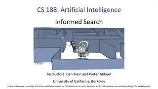
AI: Representation and Problem Solving Agents and Search Instructors: Tuomas Sandholm and Vince Conitzer Slide credits: CMU AI, http://ai.berkeley.edu

Today Reflex vs Planning Agents Search Problems Uninformed Search Methods Depth-First Search Breadth-First Search Uniform-Cost Search

Designing Agents An agent is an entity that perceives and acts. Characteristics of the percepts and state, environment, and action space dictate techniques for selecting actions Environment Sensors Percepts Agent ? Actuators Actions

Reflex Agents Reflex agents: Choose actions based on current/historic state Do not consider the future consequences of their actions May have memory or a model of the world s current state Consider how the world IS Can a reflex agent be rational?

Agents that Plan Ahead Planning agents: Decisions based on predicted consequences of actions Must have a transition model: how the world evolves in response to actions Must formulate a goal Consider how the world WOULD BE Spectrum of deliberativeness: Generate complete, optimal plan offline, then execute Generate a simple, greedy plan, start executing, replan when something goes wrong

Search Problems A search problem consists of: A state space For each state, a set Actions(s) of allowable actions {N, E} 1 N A transition model Result(s,a) E 1 A step cost function c(s,a,s ) A start state and a goal test A solution is a sequence of actions (a plan) which transforms the start state to a goal state

Example: Traveling in Romania State space: Cities Actions: Go to adjacent city Transition model Result(A, Go(B)) = B Step cost Distance along road link Start state: Arad Goal test: Is state == Bucharest? Solution? Oradea 71 Neamt 87 Zerind 151 75 Iasi Arad 140 92 Sibiu Fagaras 99 118 Vaslui 80 Rimnicu Vilcea Timisoara 142 211 111 Pitesti Lugoj 97 70 98 Hirsova 85 146 Mehadia 101 Urziceni 86 75 138 Bucharest 120 Drobeta 90 Eforie Craiova Giurgiu

State Space Graphs and Search Trees

State Space Graphs State space graph: A mathematical representation of a search problem Nodes are (abstracted) world configurations Arcs represent transitions resulting from actions The goal test is a set of goal nodes (maybe only one) In a state space graph, each state occurs only once! We can rarely build this full graph in memory (it s too big), but it s a useful idea

More Examples R L R L S S R R L R L R L L S S S S R L R L S S

State Space Graphs vs. Search Trees How big is its search tree (from S)? Consider this 4-state graph: S a b a G S G b G a b G a b G Important: Lots of repeated structure in the search tree!

Tree Search vs Graph Search

functionTREE_SEARCH(problem) returnsa solution, or failure initialize the frontier as a specific work list (stack, queue, priority queue) add initial state of problem to frontier loop do ifthe frontier is empty then returnfailure choose a node and remove it from the frontier ifthe node contains a goal state then returnthe corresponding solution for each resulting child from node add child to the frontier

functionGRAPH_SEARCH(problem) returnsa solution, or failure initialize the explored set to be empty initialize the frontier as a specific work list (stack, queue, priority queue) add initial state of problem to frontier loop do ifthe frontier is empty then returnfailure choose a node and remove it from the frontier ifthe node contains a goal state then returnthe corresponding solution add the node state to the explored set for each resulting child from node if the child state is not already in the frontier or explored set then add child to the frontier

Poll 1 What is the relationship between these sets of states after each loop iteration in GRAPH_SEARCH? (Loop invariants!!!) A B C Explored Never Seen Explored Never Seen Explored Never Seen Frontier Frontier Frontier

Graph Search This graph search algorithm overlays a tree on a graph The frontier states separate the explored states from never seen states Images: AIMA, Figure 3.8, 3.9

A Note on Implementation Nodes have state, parent, action, path-cost PARENT A child of node by action a has state = result(node.state,a) parent = node action = a path-cost = node.path_cost + step_cost(node.state, a, self.state) Node ACTION = Right PATH-COST = 6 5 5 4 4 6 6 1 1 8 8 STATE 7 7 3 3 2 2 Extract solution by tracing back parent pointers, collecting actions

BFS vs DFS

G Walk-through BFS Graph Search a c b e d f S h p r q

G Walk-through DFS Graph Search a c b e d f S h p r q

Depth-First (Tree) Search G Strategy: expand a deepest node first a a c c b b e e Implementation: Frontier is a LIFO stack d d f f S h h p p r r q q S e p d q e h r b c h r p q f a a q c G p q f a q c G a

BFS vs DFS When will BFS outperform DFS? When will DFS outperform BFS?

Search Algorithm Properties

Search Algorithm Properties Complete: Guaranteed to find a solution if one exists? Optimal: Guaranteed to find the least cost path? Time complexity? Space complexity? 1 node b nodes b2 nodes b Cartoon of search tree: b is the branching factor m is the maximum depth solutions at various depths m tiers bm nodes Number of nodes in entire tree? 1 + b + b2+ . bm = O(bm)

Search Algorithm Properties Complete: Guaranteed to find a solution if one exists? Optimal: Guaranteed to find the least cost path? Time complexity? Space complexity? 1 node b nodes b2 nodes b Cartoon of search tree: b is the branching factor m is the maximum depth solutions at various depths m tiers bm nodes Number of nodes in entire tree? 1 + b + b2+ . bm = O(bm)

Think about it 1 node b nodes b2 nodes b Are these the properties for BFS or DFS? m tiers Takes O(bm) time Uses O(bm) space on frontier bm nodes Complete with graph search & finite number of states Not optimal unless all goals are in the same level (and the same step cost everywhere)

Depth-First Search (DFS) Properties What nodes does DFS expand? Some left prefix of the tree. Could process the whole tree! If m is finite, takes time O(bm) 1 node b nodes b2 nodes b How much space does the frontier take? Only has siblings on path to root, so O(bm) m tiers Is it complete? (always find a solution) m could be infinite, so only if there are finitely many possible states and we prevent cycles (graph search) bm nodes Is it optimal? (solution is best ) No, it finds the leftmost solution, regardless of depth or cost

Breadth-First Search (BFS) Properties What nodes does BFS expand? Processes all nodes above shallowest solution Let depth of shallowest solution be s Search takes time O(bs) 1 node b nodes b2 nodes b s tiers How much space does the frontier take? Has roughly the last tier, so O(bs) bs nodes Is it complete? s must be finite if a solution exists, so yes! bm nodes Is it optimal? Only if costs are all the same (more on costs later)

Iterative Deepening Idea: get DFS s space advantage with BFS s time / shallow-solution advantages Run a DFS with depth limit 1. If no solution Run a DFS with depth limit 2. If no solution Run a DFS with depth limit 3. .. b Isn t that wastefully redundant? Generally most work happens in the lowest level searched, so not so bad!

Iterative Deepening G Strategy: expand a deepest node first to a max depth, iteratively increase the depth a c b e d f S h Implementation: Frontier is a LIFO stack p r q S e p d q e h r b c h r p q f a a q c G p q f a q c G a

Uniform Cost Search

functionGRAPH_SEARCH(problem) returnsa solution, or failure initialize the explored set to be empty initialize the frontier as a specific work list (stack, queue, priority queue) add initial state of problem to frontier loop do ifthe frontier is empty then returnfailure choose a node and remove it from the frontier ifthe node contains a goal state then returnthe corresponding solution add the node state to the explored set for each resulting child from node if the child state is not already in the frontier or explored set then add child to the frontier

functionUNIFORM-COST-SEARCH(problem) returnsa solution, or failure initialize the explored set to be empty initialize the frontier as a priority queue using node path_cost as the priority add initial state of problem to frontier with path_cost = 0 loop do ifthe frontier is empty then returnfailure choose a node and remove it from the frontier ifthe node contains a goal state then returnthe corresponding solution add the node state to the explored set for each resulting child from node if the child state is not already in the frontier or explored set then add child to the frontier else if the child is already in the frontier with higher path_cost then replace that frontier node with child

Walk-through UCS 2 C G 4 A 1 3 B S D 4 1

Summary - Reflex vs Planning Agents - Modeling state based on the problem you re trying to solve - Tree vs Graph Search - BFS, DFS, UCS - Branching factor, Search space (size of frontier) - Completeness of search is whether it will always find A solution - Optimality of search is whether it always finds the BEST solution Extra slides below on search properties and iterative deepening

Breadth-First (Tree) Search G a Strategy: expand a shallowest node first c b e Implementation: Frontier is a FIFO queue d f S h p r q S e p d Search q e h r b c Tiers h r p q f a a q c G p q f a q c G a

Uniform Cost (Tree) Search 2 G a Strategy: expand a cheapest node first: c b 8 1 2 2 e 3 d f 2 9 Frontier is a priority queue (priority: cumulative cost) 8 S h 1 1 p r q 15 0 S 1 9 e p 3 d 16 q 11 5 17 e h r 4 b c 11 Cost contours 7 6 13 h r p q f a a q c 8 G p q f a q c 11 10 G a

Uniform Cost Search (UCS) Properties What nodes does UCS expand? Processes all nodes with cost less than cheapest solution! If that solution costs C* and arcs cost at least ,then the effective depth is roughly C*/ Takes time O(bC*/ ) (exponential in effective depth) b c 1 How much space does the frontier take? Has roughly the last tier, so O(bC*/ ) c 2 C*/ tiers c 3 Is it complete? Assuming best solution has a finite cost and minimum arc cost is positive, yes! Is it optimal? Yes! (Proof next lecture via A*)

Uniform Cost Issues Remember: UCS explores increasing cost contours c 1 c 2 c 3 The good: UCS is complete and optimal! The bad: Explores options in every direction No information about goal location Start Goal We ll fix that soon!