Spiking Neurons and Spiking Neural Networks
1
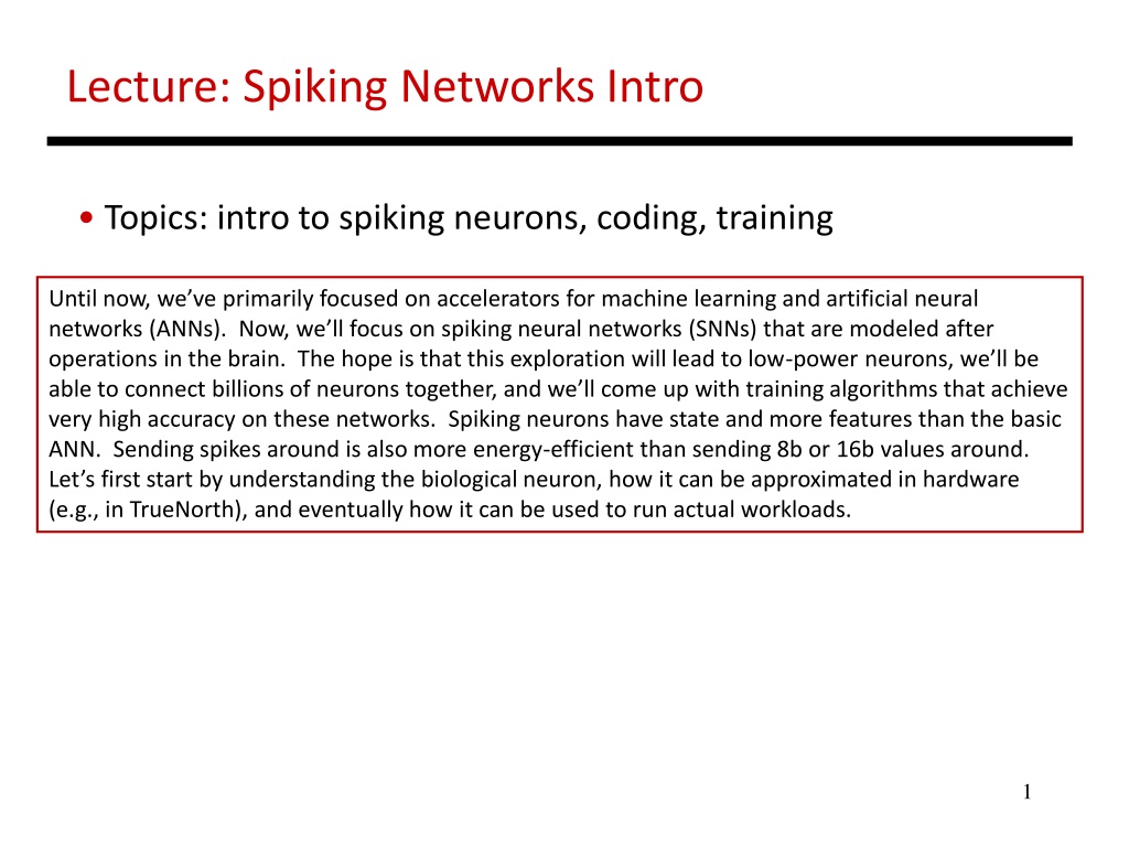
Lecture: Spiking Networks Intro
•
Topics: intro to spiking neurons, coding, training
Until now, we’ve primarily focused on accelerators for machine learning and artificial neural
networks (ANNs). Now, we’ll focus on spiking neural networks (SNNs) that are modeled after
operations in the brain. The hope is that this exploration will lead to low-power neurons, we’ll be
able to connect billions of neurons together, and we’ll come up with training algorithms that achieve
very high accuracy on these networks. Spiking neurons have state and more features than the basic
ANN. Sending spikes around is also more energy-efficient than sending 8b or 16b values around.
Let’s first start by understanding the biological neuron, how it can be approximated in hardware
(e.g., in TrueNorth), and eventually how it can be used to run actual workloads.
2
Biological Neuron
Source: stackexchange.com
The axon is the output of a neuron. Through a synapse, it connects
to the dendrite (input) of the “post-synaptic” neuron. When a
spike shows up, neurotransmitters jump across the synaptic cleft;
receptors in the post-synaptic neuron accordingly open up ionic
channels; there are Na, K, and Cl ionic channels. As a result of
these channels opening, the potential of the neuron
increases/decreases. When the potential reaches a threshold, a
spike is produced and the neuron potential drops.
3
Biological Neuron
Source: stackexchange.com
After the spike, ionic channels remain open for a “refractory
period”. During this time, incoming spikes have no impact on the
potential, so inputs are being ignored. When input spikes are
absent, the potential leaks towards a resting potential. The next
slide has a few other numerical details.
4
Biological Neuron
•
Input = dendrite; output = axon; connection = synapse
•
Neurotransmitters flow across the synaptic cleft; the receiving
(post-synaptic) neuron opens up ion channels, allowing extracellular
ions to flow in and impact membrane potential
•
Synapses can be excitatory or inhibitory
•
The neuron fires when its potential reaches a threshold;
output spike lasts 1-2ms and is about 100mV
•
Resting potential is -65mV; the threshold is typically 20-30mV higher;
each input spike raises the potential by about 1mV; need 20-50
input spikes to trigger an output spike
•
After an output spike, the potential falls below the resting potential
•
After an output spike, channels remain open for a refractory period;
during this time, input spikes have a very small impact on potential
•
A single neuron may connect to >10K other neurons; ~100 billion
neurons in human brains; ~500 trillion synapses
5
Neuron Models
•
Hodgkin and Huxley took many measurements on a
giant axon of a squid; that led to differential equations
to quantify how ion flow impacts neuron potential
•
Several experiments since then to better understand
neuronal behavior, e.g., there are different kinds of
neurons that respond differently to the same stimulus
In fact, Izhikevich has summarized 20 different neuronal behaviors. Biologically faithful architectures
strive to efficiently emulate these 20 neuron types.
6
Red Herring
•
Some detail is good, e.g., some neurons have adapted
themselves in a certain way because it’s computationally
more powerful (the refractory period, neurons that act as
integrators vs. neurons that look for a resonant input
frequency)
•
Some detail is unhelpful, e.g., complicated equations that
capture the non-idealities of bio-chemical processes (the
refractory period, the exact shape of the potential curve)
While the neuron evolves to do something very useful, we shouldn’t look at every neuron trait as
being useful; some neuron traits are because of the limitations imposed by biochemistry. The
computational power of each neuron trait remains an open problem, making things harder for
hardware designers.
7
The LIF Model
Source: Nere et al., HPCA’13
Also note Linear LIF
The most popular neuron model is linear-leaky-
integrate-fire (LLIF). When input spikes show up,
the potential is incremented/decremented
based on the synaptic weight for that input.
When inputs are absent, a leak is subtracted. In
LLIF, the increments/decrements are step
functions (unlike the smooth curves in this
figure). There’s a threshold potential, reset
potential, and a resting potential (typically 0).
8
Neuronal Codes
Source: Kruger and Aiple, 1988
In real experiments, the following
spike trains have been observed
for a collection of 30 neurons. A
key question is: what is the
information content in these
spike trains? How is information
encoded? There are multiple
encoding schemes that have been
considered and that may have a
biological basis. The two most
common ones are rate codes and
temporal codes (the latter is also
referred to as a spike code). A
rate code maps each input value
into a spike frequency. Inputs are
provided during an input window,
which is often 350 cycles or 500
cycles (1 cycle is typically 1ms).
By having 0 to 500 spikes in that
window (at most 1 spike per
cycle), we can encode 500
different input values.
9
Neuronal Codes
Source: Kruger and Aiple, 1988
On the other hand, a temporal
code (spike code) sends a single
spike within the input window.
The timing of the spike carries the
input value. We’ll discuss the
trade-offs between these codes
on a later slide. The spikes can
also have a stochastic element to
them. For example, a rate code
does not always show up as a
fixed pattern. The rate may
simply determine the probability
of a spike in any given cycle.
More recently, it is becoming
clear that temporal codes do
better when the input interval is
short, like about 16 cycles.
10
Rate Vs. Temporal Codes
•
Rate code: information is carried in terms of the frequency
of spikes
relative timing of spikes on two
dendrites is irrelevant
•
Temporal code: information is carried in terms of the exact
time of a spike (time to first spike or a phase code)
•
There are experiments that have observed both codes
•
The same code can apply throughout a multi-layer network;
the code can incorporate stochastic elements; a new input
is presented after a “phase” expires
11
Rate Codes
•
The most popular approach today
•
Output freq = w1*input freq1 + w2*input freq2
•
Works fine with integrator neurons; will also work fine
with neurons that look for resonant frequencies
•
Needs multiple spikes to encode a value (more energy)
This example shows a rate code. Let’s say the first input to the neuron is carrying the value “red” with
about 8 spikes per input window (the input window is within consecutive blue lines), and the second
input is carrying the value “blue” with about 4 spikes per window. The rate of the input spikes dictates
how the potential rises and how quickly it reaches the threshold and the output spike rate (5-6 spikes
per window). In essence, the output frequency can be expressed as a linear weighted combination of
the input frequencies. Given that the neuron equation is very much like that of an ANN, training
approaches that work for ANNs can also be applied here. Not surprisingly, most studies use rate coding
and show competitive accuracies with it. The obvious disadvantage is that we need multiple spikes to
encode any value, and likewise, multiple adds to process those spikes.
12
Temporal (Spike) Codes
•
Works fine with integrator neurons
•
What separates two different input values is the
intervening leak
•
Identifies the tail end of a weighted cluster of inputs
(also a useful way to find correlations, but it’s not the
neural network equation we know)
•
Needs a single spike to encode a value (less energy)
Temporal codes on the other hand are attractive because they reduce the spike rate (low computation
and communication energy). But an output spike represents the tail end of a weighted cluster of input
spikes. This is a reasonable way to look for patterns in inputs. But it’s not the good old ANN equation we
love and understand. So new learning techniques will have to be developed. At the moment, not much
exists in this area; I believe it’s a promising area for future work.
13
Rate Vs. Temporal Codes
Time
In 1
In 2
Potential
Output
50
125
Temporal Codes
(a) Single red spike
In 1
In 2
Potential
Output
(b) Red and pink spikes
14
Rate Vs. Temporal Codes
In 1
In 2
Potential
Output
(c) Blue and cyan spikes
In 1
In 2
Potential
Output
(d) Red and blue spikes
Temporal Codes
15
Rate Vs. Temporal Codes
In 1
In 2
Potential
Output
(e) Red and blue spikes
Rate Codes
In 1
In 2
Potential
Output
(d) Red and blue spikes
Temporal Codes
16
Training
•
Can use back-prop and supervised learning (has yielded
the best results so far)
•
More biologically feasible: Spike Timing Dependent
Plasticity (STDP)
•
If a presynaptic spike triggers a postsynaptic spike,
strengthen that synapse
•
This is an example of unsupervised learning; the network
is being trained to recognize certain clusters of inputs
SNNs can be trained with back-propagation even though it is not rooted in biology. Some of the best
results today are with back-prop and rate coding (similar to ANNs). For a more biological approach, one
can also train with STDP. With STDP, if an input spike led to an output spike, that input’s weight is
increased. If an input spike arrives soon after an output spike, that input’s weight is decreased. The
increment/decrement values depend on when the input spikes arrived (see curve on the next slide).
17
STDP
Source: Scholarpedia.org
STDP is a form of unsupervised learning.
Note that the weight adjustments are not
based on whether the final output was
correct or not. The weight adjustments
happen independently within each neuron
and do not require labeled inputs. Over
time, some output neuron gets trained to
recognize a certain pattern. A post-
processing step can label that neuron as
recognizing a certain type of output. A good
thing about STDP is that training can happen
at relatively low cost at run-time.
18
The Spiking Approach
•
Low energy for computation: only adds, no multiplies
•
Low energy for communication: depends on spikes per signal
•
Neurons have state, inputs arrive asynchronously, info
in relative timing of spikes, other biological phenomena, …
Recall that we are pursuing SNNs because of the potential for low computation and communication
energy. They also have the potential for higher accuracy because neurons have state, the spike trains
potentially carry more information, there are other biological phenomena at play that may help
(stochasticity, refractory period, leak, etc.).
19
IBM TrueNorth
•
Product of DARPA’s SyNAPSE project
•
Largest chip made by IBM (5.4 billion transistors)
•
Based on LLIF neuron model
•
Lots of on-going projects that use TrueNorth to execute
new apps
•
Lots of limitations as well – all done purposely to reduce
area/power/complexity
We’ll first examine the most high-profile SNN project – IBM TrueNorth, funded by DARPA’s SyNAPSE
project (with half a billion dollars), and yielding IBM’s largest chip (5.4 billion transistors). See modha.org
for more details on TrueNorth (there’s plenty!). TrueNorth actively pursues a simple hardware model;
yet, the neuron model is powerful enough to exhibit a variety of behaviors. Because the model is simple,
one may have to jump through hoops to map an application to TrueNorth.
20
TrueNorth Core
The next slide shows the logical view of a TrueNorth core (tile). There are several of these on a chip. The
spikes that must be processed in a tick arrive on the left (A1 and A3 in this example, indicating that the
spikes arrive on axons (rows) 1 and 3. The neurons are in the bottom row. The spike on A3 should be
seen by all the neurons that are connected to that axon. The grid is essentially storing bits to indicate if
that input axon is connected to that neuron. In addition, each point on the grid should also store the
synaptic weight for that connection. That would be pretty expensive. So to reduce the weight storage
requirement, each neuron only stores 4 weights. These weights can be roughly classified as being
Strongly Excitatory (say, a weight between 128 and 255), Weakly Excitatory (say, a weight between 0 and
128), Weakly Inhibitory (say, between -128 and 0), and Strongly Inhibitory (say, between -255 and -128).
So all the connections for that column only need to store a 2-bit value to indicate which of the 4 weights
they should use. To further reduce the storage, all the connections in a row share the same 2-bit value.
This means that an input axon will be (say) strongly excitatory to all the neurons in that core. These are
significant constraints, but dramatically bring down the storage requirement (by 8x).
21
TrueNorth Core
22
TrueNorth Core (Axonal Approach)
23
References
•
“Cognitive Computing Building Block”, A. Cassidy et al., IJCNN’13
•
“A Digital Neurosynaptic Core Using Embedded Crossbar Memory
with 45 pJ per Spike in 45nm”, P. Merolla et al., CICC, 2011
•
“TrueNorth: Design and Tool Flow of a 65mW 1 Million Neuron
Programmable Neurosynaptic Chip”, F. Akopyan et al.,
IEEE TCAD, 2015
•
“Real-Time Scalable Cortical Computing…”, A. Cassidy et al., SC’14
•
“Spiking Neuron Models”, W. Gerstner and W. Kistler, Cambridge
University Press, 2002
Spiking neural networks (SNNs) are a new approach modeled after the brain's operations, aiming for low-power neurons, billions of connections, and high accuracy training algorithms. Spiking neurons have unique features and are more energy-efficient than traditional artificial neural networks. Explore the biological neuron's functions, synaptic connections, and how spiking neurons can be approximated in hardware. Learn about the behavior of neurons during spikes, refractory periods, and the numerical details of neural communication. Discover the potential of SNNs to revolutionize machine learning and computational efficiency.

Download Presentation

Please find below an Image/Link to download the presentation.
The content on the website is provided AS IS for your information and personal use only. It may not be sold, licensed, or shared on other websites without obtaining consent from the author.If you encounter any issues during the download, it is possible that the publisher has removed the file from their server.
You are allowed to download the files provided on this website for personal or commercial use, subject to the condition that they are used lawfully. All files are the property of their respective owners.
The content on the website is provided AS IS for your information and personal use only. It may not be sold, licensed, or shared on other websites without obtaining consent from the author.
E N D
Presentation Transcript
Lecture: Spiking Networks Intro Topics: intro to spiking neurons, coding, training Until now, we ve primarily focused on accelerators for machine learning and artificial neural networks (ANNs). Now, we ll focus on spiking neural networks (SNNs) that are modeled after operations in the brain. The hope is that this exploration will lead to low-power neurons, we ll be able to connect billions of neurons together, and we ll come up with training algorithms that achieve very high accuracy on these networks. Spiking neurons have state and more features than the basic ANN. Sending spikes around is also more energy-efficient than sending 8b or 16b values around. Let s first start by understanding the biological neuron, how it can be approximated in hardware (e.g., in TrueNorth), and eventually how it can be used to run actual workloads. 1
Biological Neuron The axon is the output of a neuron. Through a synapse, it connects to the dendrite (input) of the post-synaptic neuron. When a spike shows up, neurotransmitters jump across the synaptic cleft; receptors in the post-synaptic neuron accordingly open up ionic channels; there are Na, K, and Cl ionic channels. As a result of these channels opening, the potential of the neuron increases/decreases. When the potential reaches a threshold, a spike is produced and the neuron potential drops. 2 Source: stackexchange.com
Biological Neuron After the spike, ionic channels remain open for a refractory period . During this time, incoming spikes have no impact on the potential, so inputs are being ignored. When input spikes are absent, the potential leaks towards a resting potential. The next slide has a few other numerical details. 3 Source: stackexchange.com
Biological Neuron Input = dendrite; output = axon; connection = synapse Neurotransmitters flow across the synaptic cleft; the receiving (post-synaptic) neuron opens up ion channels, allowing extracellular ions to flow in and impact membrane potential Synapses can be excitatory or inhibitory The neuron fires when its potential reaches a threshold; output spike lasts 1-2ms and is about 100mV Resting potential is -65mV; the threshold is typically 20-30mV higher; each input spike raises the potential by about 1mV; need 20-50 input spikes to trigger an output spike After an output spike, the potential falls below the resting potential After an output spike, channels remain open for a refractory period; during this time, input spikes have a very small impact on potential A single neuron may connect to >10K other neurons; ~100 billion neurons in human brains; ~500 trillion synapses 4
Neuron Models Hodgkin and Huxley took many measurements on a giant axon of a squid; that led to differential equations to quantify how ion flow impacts neuron potential Several experiments since then to better understand neuronal behavior, e.g., there are different kinds of neurons that respond differently to the same stimulus In fact, Izhikevich has summarized 20 different neuronal behaviors. Biologically faithful architectures strive to efficiently emulate these 20 neuron types. 5
Red Herring Some detail is good, e.g., some neurons have adapted themselves in a certain way because it s computationally more powerful (the refractory period, neurons that act as integrators vs. neurons that look for a resonant input frequency) Some detail is unhelpful, e.g., complicated equations that capture the non-idealities of bio-chemical processes (the refractory period, the exact shape of the potential curve) While the neuron evolves to do something very useful, we shouldn t look at every neuron trait as being useful; some neuron traits are because of the limitations imposed by biochemistry. The computational power of each neuron trait remains an open problem, making things harder for hardware designers. 6
The LIF Model Also note Linear LIF The most popular neuron model is linear-leaky- integrate-fire (LLIF). When input spikes show up, the potential is incremented/decremented based on the synaptic weight for that input. When inputs are absent, a leak is subtracted. In LLIF, the increments/decrements are step functions (unlike the smooth curves in this figure). There s a threshold potential, reset potential, and a resting potential (typically 0). 7 Source: Nere et al., HPCA 13
Neuronal Codes In real experiments, the following spike trains have been observed for a collection of 30 neurons. A key question is: what is the information content in these spike trains? How is information encoded? There are multiple encoding schemes that have been considered and that may have a biological basis. The two most common ones are rate codes and temporal codes (the latter is also referred to as a spike code). A rate code maps each input value into a spike frequency. Inputs are provided during an input window, which is often 350 cycles or 500 cycles (1 cycle is typically 1ms). By having 0 to 500 spikes in that window (at most 1 spike per cycle), we can encode 500 different input values. 8 Source: Kruger and Aiple, 1988
Neuronal Codes On the other hand, a temporal code (spike code) sends a single spike within the input window. The timing of the spike carries the input value. We ll discuss the trade-offs between these codes on a later slide. The spikes can also have a stochastic element to them. For example, a rate code does not always show up as a fixed pattern. The rate may simply determine the probability of a spike in any given cycle. More recently, it is becoming clear that temporal codes do better when the input interval is short, like about 16 cycles. 9 Source: Kruger and Aiple, 1988
Rate Vs. Temporal Codes Rate code: information is carried in terms of the frequency of spikes relative timing of spikes on two dendrites is irrelevant Temporal code: information is carried in terms of the exact time of a spike (time to first spike or a phase code) There are experiments that have observed both codes The same code can apply throughout a multi-layer network; the code can incorporate stochastic elements; a new input is presented after a phase expires 10
Rate Codes The most popular approach today Output freq = w1*input freq1 + w2*input freq2 Works fine with integrator neurons; will also work fine with neurons that look for resonant frequencies Needs multiple spikes to encode a value (more energy) This example shows a rate code. Let s say the first input to the neuron is carrying the value red with about 8 spikes per input window (the input window is within consecutive blue lines), and the second input is carrying the value blue with about 4 spikes per window. The rate of the input spikes dictates how the potential rises and how quickly it reaches the threshold and the output spike rate (5-6 spikes per window). In essence, the output frequency can be expressed as a linear weighted combination of the input frequencies. Given that the neuron equation is very much like that of an ANN, training approaches that work for ANNs can also be applied here. Not surprisingly, most studies use rate coding and show competitive accuracies with it. The obvious disadvantage is that we need multiple spikes to encode any value, and likewise, multiple adds to process those spikes. 11
Temporal (Spike) Codes Works fine with integrator neurons What separates two different input values is the intervening leak Identifies the tail end of a weighted cluster of inputs (also a useful way to find correlations, but it s not the neural network equation we know) Needs a single spike to encode a value (less energy) Temporal codes on the other hand are attractive because they reduce the spike rate (low computation and communication energy). But an output spike represents the tail end of a weighted cluster of input spikes. This is a reasonable way to look for patterns in inputs. But it s not the good old ANN equation we love and understand. So new learning techniques will have to be developed. At the moment, not much exists in this area; I believe it s a promising area for future work. 12
Rate Vs. Temporal Codes Temporal Codes Time 125 50 (a) Single red spike In 1 In 2 Potential Output (b) Red and pink spikes In 1 In 2 Potential Output 13
Rate Vs. Temporal Codes Temporal Codes (c) Blue and cyan spikes In 1 In 2 Potential Output (d) Red and blue spikes In 1 In 2 Potential Output 14
Rate Vs. Temporal Codes Temporal Codes (d) Red and blue spikes In 1 In 2 Potential Output Rate Codes (e) Red and blue spikes In 1 In 2 Potential Output 15
Training Can use back-prop and supervised learning (has yielded the best results so far) More biologically feasible: Spike Timing Dependent Plasticity (STDP) If a presynaptic spike triggers a postsynaptic spike, strengthen that synapse This is an example of unsupervised learning; the network is being trained to recognize certain clusters of inputs SNNs can be trained with back-propagation even though it is not rooted in biology. Some of the best results today are with back-prop and rate coding (similar to ANNs). For a more biological approach, one can also train with STDP. With STDP, if an input spike led to an output spike, that input s weight is increased. If an input spike arrives soon after an output spike, that input s weight is decreased. The increment/decrement values depend on when the input spikes arrived (see curve on the next slide). 16
STDP STDP is a form of unsupervised learning. Note that the weight adjustments are not based on whether the final output was correct or not. The weight adjustments happen independently within each neuron and do not require labeled inputs. Over time, some output neuron gets trained to recognize a certain pattern. A post- processing step can label that neuron as recognizing a certain type of output. A good thing about STDP is that training can happen at relatively low cost at run-time. 17 Source: Scholarpedia.org
The Spiking Approach Low energy for computation: only adds, no multiplies Low energy for communication: depends on spikes per signal Neurons have state, inputs arrive asynchronously, info in relative timing of spikes, other biological phenomena, Recall that we are pursuing SNNs because of the potential for low computation and communication energy. They also have the potential for higher accuracy because neurons have state, the spike trains potentially carry more information, there are other biological phenomena at play that may help (stochasticity, refractory period, leak, etc.). 18
IBM TrueNorth Product of DARPA s SyNAPSE project Largest chip made by IBM (5.4 billion transistors) Based on LLIF neuron model Lots of on-going projects that use TrueNorth to execute new apps Lots of limitations as well all done purposely to reduce area/power/complexity We ll first examine the most high-profile SNN project IBM TrueNorth, funded by DARPA s SyNAPSE project (with half a billion dollars), and yielding IBM s largest chip (5.4 billion transistors). See modha.org for more details on TrueNorth (there s plenty!). TrueNorth actively pursues a simple hardware model; yet, the neuron model is powerful enough to exhibit a variety of behaviors. Because the model is simple, one may have to jump through hoops to map an application to TrueNorth. 19
TrueNorth Core The next slide shows the logical view of a TrueNorth core (tile). There are several of these on a chip. The spikes that must be processed in a tick arrive on the left (A1 and A3 in this example, indicating that the spikes arrive on axons (rows) 1 and 3. The neurons are in the bottom row. The spike on A3 should be seen by all the neurons that are connected to that axon. The grid is essentially storing bits to indicate if that input axon is connected to that neuron. In addition, each point on the grid should also store the synaptic weight for that connection. That would be pretty expensive. So to reduce the weight storage requirement, each neuron only stores 4 weights. These weights can be roughly classified as being Strongly Excitatory (say, a weight between 128 and 255), Weakly Excitatory (say, a weight between 0 and 128), Weakly Inhibitory (say, between -128 and 0), and Strongly Inhibitory (say, between -255 and -128). So all the connections for that column only need to store a 2-bit value to indicate which of the 4 weights they should use. To further reduce the storage, all the connections in a row share the same 2-bit value. This means that an input axon will be (say) strongly excitatory to all the neurons in that core. These are significant constraints, but dramatically bring down the storage requirement (by 8x). 20
References Cognitive Computing Building Block , A. Cassidy et al., IJCNN 13 A Digital Neurosynaptic Core Using Embedded Crossbar Memory with 45 pJ per Spike in 45nm , P. Merolla et al., CICC, 2011 TrueNorth: Design and Tool Flow of a 65mW 1 Million Neuron Programmable Neurosynaptic Chip , F. Akopyan et al., IEEE TCAD, 2015 Real-Time Scalable Cortical Computing , A. Cassidy et al., SC 14 Spiking Neuron Models , W. Gerstner and W. Kistler, Cambridge University Press, 2002 23


 Codes")


")