Hopfield Nets in Neural Networks


Neural Networks for Machine Learning
Lecture 11a
Hopfield Nets
Hopfield Nets
•
A Hopfield net is composed of
binary threshold units with
recurrent connections between
them.
•
Recurrent networks of non-
linear units are generally very
hard to analyze. They can
behave in many different ways:
–
Settle to a stable state
–
Oscillate
–
Follow chaotic trajectories
that cannot be predicted far
into the future.
•
B
u
t
J
o
h
n
H
o
p
f
i
e
l
d
(
a
n
d
o
t
h
e
r
s
)
r
e
a
l
i
z
e
d
t
h
a
t
i
f
t
h
e
c
o
n
n
e
c
t
i
o
n
s
a
r
e
s
y
m
m
e
t
r
i
c
,
t
h
e
r
e
i
s
a
g
l
o
b
a
l
e
n
e
r
g
y
f
u
n
c
t
i
o
n
.
–
Each binary
“
configuration
”
of the whole network has an
energy.
–
The binary threshold
decision rule causes the
network to settle to a
minimum of this energy
function.
The energy function
•
The global energy is the sum of many contributions. Each contribution
depends on
one connection weight
and the binary states of
two
neurons:
•
T
h
i
s
s
i
m
p
l
e
q
u
a
d
r
a
t
i
c
e
n
e
r
g
y
f
u
n
c
t
i
o
n
m
a
k
e
s
i
t
p
o
s
s
i
b
l
e
f
o
r
e
a
c
h
u
n
i
t
t
o
c
o
m
p
u
t
e
l
o
c
a
l
l
y
h
o
w
i
t
’
s
s
t
a
t
e
a
f
f
e
c
t
s
t
h
e
g
l
o
b
a
l
e
n
e
r
g
y
:
Settling to an energy minimum
•
To find an energy minimum in this
net, start from a random state and
then update units
one at a time
in
random order.
–
Update each unit to whichever
of its two states gives the
lowest global energy.
–
i.e.
use binary threshold units.
3 2 3 3
-1
-4
-1
1
1
0
0
?
0
- E = goodness = 3
Settling to an energy minimum
•
To find an energy minimum in this
net, start from a random state and
then update units
one at a time
in
random order.
–
Update each unit to whichever
of its two states gives the
lowest global energy.
–
i.e.
use binary threshold units.
3 2 3 3
-1
-4
-1
1
1
0
0
0
?
- E = goodness = 3
Settling to an energy minimum
•
To find an energy minimum in this
net, start from a random state and
then update units
one at a time
in
random order.
–
Update each unit to whichever
of its two states gives the
lowest global energy.
–
i.e.
use binary threshold units.
3 2 3 3
-1
-4
1
-1
1
1
0
0
0
?
- E = goodness = 3
- E = goodness = 4
A deeper energy minimum
•
The net has two triangles in which the
three units mostly support each other.
–
Each triangle mostly hates the other
triangle.
•
The triangle on the left differs from the
one on the right by having a weight of 2
where the other one has a weight of 3.
–
So turning on the units in the triangle
on the right gives the deepest
minimum.
3 2 3 3
-1
-4
1
-1
1
1
0
0
- E = goodness = 5
Why do the decisions need to be sequential?
•
If units make
simultaneous
decisions the energy could go up.
•
With simultaneous parallel updating
we can get oscillations.
–
They always have a period of 2.
•
If the updates occur in parallel but
with random timing, the oscillations
are usually destroyed.
-100
+5
+5
0
0
At the next parallel step, both
units will turn on. This has
very high energy, so then
they will both turn off again.
A neat way to make use of this type of computation
•
Hopfield (1982) proposed that
memories could be energy
minima of a neural net.
–
The binary threshold decision
rule can then be used to
“
clean up
”
incomplete or
corrupted memories.
•
The idea of memories as energy
minima was proposed by I. A.
Richards in 1924 in “Principles of
Literary Criticism”.
•
Using energy minima to
represent memories gives a
content-addressable memory:
–
An item can be accessed
by just knowing part of its
content.
•
This was really amazing
in the year 16 BG.
–
It is robust against
hardware damage.
–
It’s like reconstructing a
dinosaur from a few bones.
Storing memories in a Hopfield net
•
If we use activities of 1 and -1,
we can store a binary state
vector by incrementing the
weight between any two units by
the product of their activities.
–
We treat biases as weights
from a permanently on unit.
•
With states of 0 and 1 the rule is
slightly more complicated.
This is a very simple rule
that is not error-driven.
That is both its strength
and its weakness
Neural Networks for Machine Learning
Lecture 11b
Dealing with spurious minima in Hopfield Nets
The storage capacity of a Hopfield net
•
Using Hopfield
’
s storage rule
the capacity of a totally
connected net with N units is
only about 0.15N memories.
–
At
N
bits per memory this is
only bits.
–
This does not make
efficient use of the bits
required to store the
weights.
•
The net has weights and
biases.
•
After storing M memories,
each connection weight has an
integer value in the range
[–M, M].
•
So the number of bits required
to store the weights and biases
is:
Spurious minima limit capacity
•
Each time we memorize a
configuration, we hope to
create a new energy minimum.
–
But what if two nearby
minima merge to create a
minimum at an
intermediate location?
–
This limits the capacity of a
Hopfield net.
The state space is the corners of a
hypercube. Showing it as a 1-D
continuous space is a misrepresentation.
Avoiding spurious minima by unlearning
•
Hopfield, Feinstein and Palmer
suggested the following
strategy:
–
Let the net settle from a
random initial state and then
do
un
learning.
–
This will get rid of deep,
spurious minima and
increase memory capacity.
•
They showed that this worked.
–
But they had no analysis.
•
Crick and Mitchison proposed
unlearning as a model of what
dreams are for.
–
That
’
s why you don
’
t
remember them
(unless you
wake up during the dream)
•
But how much unlearning should
we do?
–
Can we derive unlearning as
the right way to minimize
some cost function?
Increasing the capacity of a Hopfield net
•
Physicists love the idea that the
math they already know might
explain how the brain works.
–
Many papers were published in
physics journals about Hopfield
nets and their storage capacity.
•
Eventually, Elizabeth Gardiner
figured out that there was a much
better storage rule that uses the
full capacity of the weights.
•
Instead of trying to store vectors in
one shot, cycle through the training
set many times.
–
Use the perceptron
convergence procedure to train
each unit to have the correct
state given the states of all the
other units in that vector.
•
Statisticians call this technique
“pseudo-likelihood”.
Neural Networks for Machine Learning
Lecture 11c
Hopfield Nets with hidden units
A different computational role for Hopfield nets
•
Instead of using the net to store
memories, use it to construct
interpretations of sensory input.
–
The input is represented by the
visible units.
–
The interpretation is represented
by the states of the hidden units.
–
The badness of the interpretation
is represented by the energy.
visible units
hidden units
What can we infer about 3-D edges from 2-D lines
in an image?
•
A 2-D line in an image could have
been caused by many different 3-D
edges in the world.
•
If we assume it
’
s a straight 3-D edge,
the information that has been lost in
the image is the 3-D depth of each
end of the 2-D line.
–
So there is a family of 3-D edges
that all correspond to the same
2-D line.
You can only see one
of these 3-D edges at
a time because they
occlude one another.
An example: Interpreting a line drawing
•
Use one
“
2-D line
”
unit for each
possible line in the picture.
–
Any particular picture will
only activate a very small
subset of the line units
.
•
Use one
“
3-D line
”
unit for each
possible 3-D line in the scene.
–
Each 2-D line unit could be
the projection of many
possible 3-D lines. Make
these 3-D lines
compete
.
•
Make 3-D lines
support
each
other if they join in 3-D.
•
M
a
k
e
t
h
e
m
s
t
r
o
n
g
l
y
s
u
p
p
o
r
t
e
a
c
h
o
t
h
e
r
i
f
t
h
e
y
j
o
i
n
a
t
r
i
g
h
t
a
n
g
l
e
s
.
Join in 3-D
Join in 3-D
at right angle
2-D lines
3-D lines
picture
Two difficult computational issues
•
Using the states of the hidden units
to represent an interpretation of the
input raises two difficult issues:
–
Search (lecture 11)
How do we
avoid getting trapped in poor
local minima of the energy
function?
•
Poor minima represent sub-
optimal interpretations.
–
Learning (lecture 12)
How do we
learn the weights on the
connections to the hidden units
and between the hidden units?
Neural Networks for Machine Learning
Lecture 11d
Using stochastic units to improve search
No
isy networks find better energy minima
•
A Hopfield net always makes decisions that reduce the energy.
–
This makes it impossible to escape from local minima.
•
We can use random noise to escape from poor minima.
–
Start with a lot of noise so its easy to cross energy barriers.
–
Slowly reduce the noise so that the system ends up in a deep
minimum. This is
“
simulated annealing
”
(Kirkpatrick et.al. 1981)
A B C
How temperature affects transition probabilities
A
B
A
B
High temperature
transition
probabilities
Low temperature
transition
probabilities
Stochastic binary units
•
Replace the binary threshold units by binary stochastic units that
make biased random decisions.
–
The
“
temperature
”
controls the amount of noise
–
Raising the noise level is equivalent to decreasing all the energy
gaps between configurations.
temperature
Simulated annealing is a distraction
•
Simulated annealing is a powerful method for improving searches
that get stuck in local optima.
•
It was one of the ideas that led to Boltzmann machines.
•
But it
’
s a big distraction from the main ideas behind Boltzmann
machines.
–
So it will not be covered in this course.
–
From now on, we will use binary stochastic units that have a
temperature of 1.
Thermal equilibrium at a temperature of 1
•
Thermal equilibrium is a difficult
concept!
–
Reaching thermal equilibrium
does not mean that the system
has settled down into the
lowest energy configuration.
–
The thing that settles down is
the
probability distribution
over
configurations.
–
This settles to the stationary
distribution.
•
There is a nice intuitive way to
think about thermal
equilibrium:
–
Imagine a huge ensemble
of systems that all have
exactly the same energy
function.
–
The probability of a
configuration is just the
fraction of the systems that
have that configuration.
Approaching thermal equilibrium
•
We start with any distribution we like over all the identical systems.
–
We could start with all the systems in the same configuration.
–
Or with an equal number of systems in each possible configuration.
•
Then we keep applying our stochastic update rule to pick the next
configuration for each individual system.
•
After running the systems stochastically in the right way, we may
eventually reach a situation where the fraction of systems in each
configuration remains constant.
–
This is the stationary distribution that physicists call thermal
equilibrium.
–
Any given system keeps changing its configuration, but the fraction
of systems in each configuration does not change.
An analogy
•
Imagine a casino in Las Vegas that is full of card dealers (we need
many more than 52! of them).
•
We start with all the card packs in standard order and then the dealers
all start shuffling their packs.
–
After a few time steps, the king of spades still has a good chance
of being next to the queen of spades. The packs have not yet
forgotten where they started.
–
After prolonged shuffling, the packs will have forgotten where they
started. There will be an equal number of packs in each of the 52!
possible orders.
–
Once equilibrium has been reached, the number of packs that
leave a configuration at each time step will be equal to the number
that enter the configuration.
•
The only thing wrong with this analogy is that all the configurations
have equal energy, so they all end up with the same probability.
Neural Networks for Machine Learning
Lecture 11e
How a Boltzmann Machine models data
Modeling binary data
•
Given a training set of binary vectors, fit a model that will assign a
probability to every possible binary vector.
–
This is useful for deciding if other binary vectors come from the
same distribution (
e.g.
documents represented by binary
features that represents the occurrence of a particular word).
–
It can be used for monitoring complex systems to detect unusual
behavior.
–
If we have models of several different distributions it can be used
to compute the posterior probability that a particular distribution
produced the observed data.
How a causal model generates data
•
In a causal model we generate data
in two sequential steps:
–
First pick the hidden states from
their prior distribution.
–
Then pick the visible states from
their conditional distribution given
the hidden states.
•
The probability of generating a visible
vector, v, is computed by summing
over all possible hidden states. Each
hidden state is an “explanation” of v.
hidden
visible
1
1
1
0
0
How a Boltzmann Machine generates data
•
It is
not
a causal generative model.
•
Instead, everything is defined in terms of the energies of joint
configurations of the visible and hidden units.
•
The energies of joint configurations are related to their probabilities
in two ways.
–
We can simply define the probability to be
–
Alternatively, we can define the probability to be the probability
of finding the network in that joint configuration after we have
updated all of the stochastic binary units many times.
•
These two definitions agree.
The Energy of a joint configuration
bias of
unit k
weight between
visible unit i and
hidden unit k
E
n
e
r
g
y
w
i
t
h
c
o
n
f
i
g
u
r
a
t
i
o
n
v
o
n
t
h
e
v
i
s
i
b
l
e
u
n
i
t
s
a
n
d
h
o
n
t
h
e
h
i
d
d
e
n
u
n
i
t
s
b
i
n
a
r
y
s
t
a
t
e
o
f
u
n
i
t
i
i
n
v
indexes every
non-identical pair
of i and j once
Using energies to define probabilities
•
The probability of a joint configuration
over both visible and hidden units
depends on the energy of that joint
configuration compared with the
energy of all other joint
configurations.
•
The probability of a configuration of
the visible units is the sum of the
probabilities of all the joint
configurations that contain it.
partition
function
h1 h2
+2 +1
v1 v2
An example of how
weights define a
distribution
1 1
1 1 2 7.39 .186
1 1
1 0 2 7.39 .186
1 1
0 1 1 2.72 .069
1 1
0 0 0 1 .025
1 0
1 1 1 2.72 .069
1 0
1 0 2 7.39 .186
1 0
0 1 0 1 .025
1 0
0 0 0 1 .025
0 1
1 1 0 1 .025
0 1
1 0 0 1 .025
0 1
0 1 1 2.72 .069
0 1
0 0 0 1 .025
0 0
1 1 -1 0.37 .009
0 0
1 0 0 1 .025
0 0
0 1 0 1 .025
0 0
0 0 0 1 .025
39.70
0.466
0.305
0.144
0.084
-1
Getting a sample from the model
•
If there are more than a few hidden
units, we cannot compute the
normalizing term (the partition
function) because it has exponentially
many terms.
•
So we use Markov Chain Monte
Carlo to get samples from the model
starting from a random global
configuration:
–
Keep picking units at random and
allowing them to stochastically
update their states based on their
energy gaps.
•
Run the Markov chain until
it reaches its stationary
distribution (thermal
equilibrium at a
temperature of 1).
–
The probability of a
global configuration is
then related to its
energy by the
Boltzmann distribution.
Getting a sample from the posterior distribution over
hidden configurations for a given data vector
•
The number of possible hidden configurations is exponential so
we need MCMC to sample from the posterior.
–
It is just the same as getting a sample from the model, except
that we keep the visible units clamped to the given data
vector.
•
Only the hidden units are allowed to change states
•
Samples from the posterior are required for learning the weights.
Each hidden configuration is an “explanation” of an observed
visible configuration. Better explanations have lower energy.
Hopfield Nets, pioneered by John Hopfield, are a type of neural network with symmetric connections and a global energy function. These networks are composed of binary threshold units with recurrent connections, making them settle into stable states based on an energy minimization process. The energy function is determined by connection weights and binary states of neurons, allowing for local computations on energy gaps. Settling to an energy minimum involves updating units one at a time to minimize global energy. Deeper energy minima in these networks can exhibit complex interactions between units.

Download Presentation

Please find below an Image/Link to download the presentation.
The content on the website is provided AS IS for your information and personal use only. It may not be sold, licensed, or shared on other websites without obtaining consent from the author.If you encounter any issues during the download, it is possible that the publisher has removed the file from their server.
You are allowed to download the files provided on this website for personal or commercial use, subject to the condition that they are used lawfully. All files are the property of their respective owners.
The content on the website is provided AS IS for your information and personal use only. It may not be sold, licensed, or shared on other websites without obtaining consent from the author.
E N D
Presentation Transcript
Neural Networks for Machine Learning Lecture 11a Hopfield Nets Geoffrey Hinton Nitish Srivastava, Kevin Swersky Tijmen Tieleman Abdel-rahman Mohamed
Hopfield Nets But John Hopfield (and others) realized that if the connections are symmetric, there is a global energy function. Each binary configuration of the whole network has an energy. The binary threshold decision rule causes the network to settle to a minimum of this energy function. A Hopfield net is composed of binary threshold units with recurrent connections between them. Recurrent networks of non- linear units are generally very hard to analyze. They can behave in many different ways: Settle to a stable state Oscillate Follow chaotic trajectories that cannot be predicted far into the future.
The energy function The global energy is the sum of many contributions. Each contribution depends on one connection weight and the binary states of two neurons: i bi- E =- si sisjwij i<j This simple quadratic energy function makes it possible for each unit to compute locally how it s state affects the global energy: j Energy gap = DEi = E(si= 0)-E(si=1) = bi+ sjwij
Settling to an energy minimum -4 To find an energy minimum in this net, start from a random state and then update units one at a time in random order. Update each unit to whichever of its two states gives the lowest global energy. i.e. use binary threshold units. 0 ? 1 3 2 3 3 -1 -1 0 0 1 - E = goodness = 3
Settling to an energy minimum -4 To find an energy minimum in this net, start from a random state and then update units one at a time in random order. Update each unit to whichever of its two states gives the lowest global energy. i.e. use binary threshold units. 0 1 3 2 3 3 -1 -1 0 0 1 ? - E = goodness = 3
Settling to an energy minimum -4 To find an energy minimum in this net, start from a random state and then update units one at a time in random order. Update each unit to whichever of its two states gives the lowest global energy. i.e. use binary threshold units. 0 1 3 2 3 3 -1 -1 1 0 ? 0 1 - E = goodness = 3 - E = goodness = 4
A deeper energy minimum The net has two triangles in which the three units mostly support each other. Each triangle mostly hates the other triangle. The triangle on the left differs from the one on the right by having a weight of 2 where the other one has a weight of 3. So turning on the units in the triangle on the right gives the deepest minimum. -4 1 0 3 2 3 3 -1 -1 1 1 0 - E = goodness = 5
Why do the decisions need to be sequential? If units make simultaneous decisions the energy could go up. With simultaneous parallel updating we can get oscillations. They always have a period of 2. If the updates occur in parallel but with random timing, the oscillations are usually destroyed. -100 0 0 +5 +5 At the next parallel step, both units will turn on. This has very high energy, so then they will both turn off again.
A neat way to make use of this type of computation Hopfield (1982) proposed that memories could be energy minima of a neural net. The binary threshold decision rule can then be used to clean up incomplete or corrupted memories. The idea of memories as energy minima was proposed by I. A. Richards in 1924 in Principles of Literary Criticism . Using energy minima to represent memories gives a content-addressable memory: An item can be accessed by just knowing part of its content. This was really amazing in the year 16 BG. It is robust against hardware damage. It s like reconstructing a dinosaur from a few bones.
Storing memories in a Hopfield net If we use activities of 1 and -1, we can store a binary state vector by incrementing the weight between any two units by the product of their activities. We treat biases as weights from a permanently on unit. Dwij=sisj This is a very simple rule that is not error-driven. That is both its strength and its weakness With states of 0 and 1 the rule is slightly more complicated. = 1 1 4 ( ( ) 2 ) w s s ij i j 2
Neural Networks for Machine Learning Lecture 11b Dealing with spurious minima in Hopfield Nets Geoffrey Hinton Nitish Srivastava, Kevin Swersky Tijmen Tieleman Abdel-rahman Mohamed
The storage capacity of a Hopfield net N2 The net has weights and biases. After storing M memories, each connection weight has an integer value in the range [ M, M]. So the number of bits required to store the weights and biases is: N2log(2M +1) Using Hopfield s storage rule the capacity of a totally connected net with N units is only about 0.15N memories. At N bits per memory this is only bits. This does not make efficient use of the bits required to store the weights. 0.15 N2
Spurious minima limit capacity Each time we memorize a configuration, we hope to create a new energy minimum. But what if two nearby minima merge to create a minimum at an intermediate location? This limits the capacity of a Hopfield net. The state space is the corners of a hypercube. Showing it as a 1-D continuous space is a misrepresentation.
Avoiding spurious minima by unlearning Hopfield, Feinstein and Palmer suggested the following strategy: Let the net settle from a random initial state and then do unlearning. This will get rid of deep, spurious minima and increase memory capacity. They showed that this worked. But they had no analysis. Crick and Mitchison proposed unlearning as a model of what dreams are for. That s why you don t remember them (unless you wake up during the dream) But how much unlearning should we do? Can we derive unlearning as the right way to minimize some cost function?
Increasing the capacity of a Hopfield net Physicists love the idea that the math they already know might explain how the brain works. Many papers were published in physics journals about Hopfield nets and their storage capacity. Eventually, Elizabeth Gardiner figured out that there was a much better storage rule that uses the full capacity of the weights. Instead of trying to store vectors in one shot, cycle through the training set many times. Use the perceptron convergence procedure to train each unit to have the correct state given the states of all the other units in that vector. Statisticians call this technique pseudo-likelihood .
Neural Networks for Machine Learning Lecture 11c Hopfield Nets with hidden units Geoffrey Hinton Nitish Srivastava, Kevin Swersky Tijmen Tieleman Abdel-rahman Mohamed
A different computational role for Hopfield nets hidden units Instead of using the net to store memories, use it to construct interpretations of sensory input. The input is represented by the visible units. The interpretation is represented by the states of the hidden units. The badness of the interpretation is represented by the energy. visible units
What can we infer about 3-D edges from 2-D lines in an image? A 2-D line in an image could have been caused by many different 3-D edges in the world. If we assume it s a straight 3-D edge, the information that has been lost in the image is the 3-D depth of each end of the 2-D line. So there is a family of 3-D edges that all correspond to the same 2-D line. You can only see one of these 3-D edges at a time because they occlude one another.
An example: Interpreting a line drawing Use one 2-D line unit for each possible line in the picture. Any particular picture will only activate a very small subset of the line units. Use one 3-D line unit for each possible 3-D line in the scene. Each 2-D line unit could be the projection of many possible 3-D lines. Make these 3-D lines compete. Make 3-D lines support each other if they join in 3-D. Make them strongly support each other if they join at right angles. 3-D lines 2-D lines picture
Two difficult computational issues Using the states of the hidden units to represent an interpretation of the input raises two difficult issues: Search (lecture 11) How do we avoid getting trapped in poor local minima of the energy function? Poor minima represent sub- optimal interpretations. Learning (lecture 12) How do we learn the weights on the connections to the hidden units and between the hidden units?
Neural Networks for Machine Learning Lecture 11d Using stochastic units to improve search Geoffrey Hinton Nitish Srivastava, Kevin Swersky Tijmen Tieleman Abdel-rahman Mohamed
Noisy networks find better energy minima A Hopfield net always makes decisions that reduce the energy. This makes it impossible to escape from local minima. We can use random noise to escape from poor minima. Start with a lot of noise so its easy to cross energy barriers. Slowly reduce the noise so that the system ends up in a deep minimum. This is simulated annealing (Kirkpatrick et.al. 1981) A B C
How temperature affects transition probabilities = ( ) 2 . 0 p A B = ( ) 1 . 0 p A B High temperature transition probabilities A B = ( ) . 0 001 p A B = ( ) 000001 . 0 p A B Low temperature transition probabilities A B
Stochastic binary units Replace the binary threshold units by binary stochastic units that make biased random decisions. The temperature controls the amount of noise Raising the noise level is equivalent to decreasing all the energy gaps between configurations. 1 p(si=1) = 1+e-DEiT temperature j Energy gap = DEi = E(si= 0)-E(si=1) = bi+ sjwij
Simulated annealing is a distraction Simulated annealing is a powerful method for improving searches that get stuck in local optima. It was one of the ideas that led to Boltzmann machines. But it s a big distraction from the main ideas behind Boltzmann machines. So it will not be covered in this course. From now on, we will use binary stochastic units that have a temperature of 1.
Thermal equilibrium at a temperature of 1 Thermal equilibrium is a difficult concept! Reaching thermal equilibrium does not mean that the system has settled down into the lowest energy configuration. The thing that settles down is the probability distribution over configurations. This settles to the stationary distribution. There is a nice intuitive way to think about thermal equilibrium: Imagine a huge ensemble of systems that all have exactly the same energy function. The probability of a configuration is just the fraction of the systems that have that configuration.
Approaching thermal equilibrium We start with any distribution we like over all the identical systems. We could start with all the systems in the same configuration. Or with an equal number of systems in each possible configuration. Then we keep applying our stochastic update rule to pick the next configuration for each individual system. After running the systems stochastically in the right way, we may eventually reach a situation where the fraction of systems in each configuration remains constant. This is the stationary distribution that physicists call thermal equilibrium. Any given system keeps changing its configuration, but the fraction of systems in each configuration does not change.
An analogy Imagine a casino in Las Vegas that is full of card dealers (we need many more than 52! of them). We start with all the card packs in standard order and then the dealers all start shuffling their packs. After a few time steps, the king of spades still has a good chance of being next to the queen of spades. The packs have not yet forgotten where they started. After prolonged shuffling, the packs will have forgotten where they started. There will be an equal number of packs in each of the 52! possible orders. Once equilibrium has been reached, the number of packs that leave a configuration at each time step will be equal to the number that enter the configuration. The only thing wrong with this analogy is that all the configurations have equal energy, so they all end up with the same probability.
Neural Networks for Machine Learning Lecture 11e How a Boltzmann Machine models data Geoffrey Hinton Nitish Srivastava, Kevin Swersky Tijmen Tieleman Abdel-rahman Mohamed
Modeling binary data Given a training set of binary vectors, fit a model that will assign a probability to every possible binary vector. This is useful for deciding if other binary vectors come from the same distribution (e.g. documents represented by binary features that represents the occurrence of a particular word). It can be used for monitoring complex systems to detect unusual behavior. If we have models of several different distributions it can be used to compute the posterior probability that a particular distribution produced the observed data. = data i Model p ) | ( ( | ) p data ( Model | i j ) p data Model j
How a causal model generates data In a causal model we generate data in two sequential steps: First pick the hidden states from their prior distribution. Then pick the visible states from their conditional distribution given the hidden states. The probability of generating a visible vector, v, is computed by summing over all possible hidden states. Each hidden state is an explanation of v. 1 0 hidden 1 1 0 visible p(v)= p(h)p(v|h) h
How a Boltzmann Machine generates data It is not a causal generative model. Instead, everything is defined in terms of the energies of joint configurations of the visible and hidden units. The energies of joint configurations are related to their probabilities in two ways. We can simply define the probability to be Alternatively, we can define the probability to be the probability of finding the network in that joint configuration after we have updated all of the stochastic binary units many times. These two definitions agree. p(v,h) e-E(v,h)
The Energy of a joint configuration bias of unit k of unit i in v binary state i,k -E(v,h)= + + + + vibi hkbk vivjwij vihkwik hkhlwkl i vis k hid i<j k<l weight between visible unit i and hidden unit k Energy with configuration v on the visible units and h on the hidden units indexes every non-identical pair of i and j once
Using energies to define probabilities e-E(v,h) e-E(u,g) u,g The probability of a joint configuration over both visible and hidden units depends on the energy of that joint configuration compared with the energy of all other joint configurations. p(v,h) = partition function e-E(v,h) e-E(u,g) u,g The probability of a configuration of the visible units is the sum of the probabilities of all the joint configurations that contain it. p(v) = h
e-E h -E p(v, h ) p(v) v An example of how weights define a distribution 1 1 1 1 2 7.39 .186 1 1 1 0 2 7.39 .186 1 1 0 1 1 2.72 .069 1 1 0 0 0 1 .025 1 0 1 1 1 2.72 .069 1 0 1 0 2 7.39 .186 1 0 0 1 0 1 .025 1 0 0 0 0 1 .025 0 1 1 1 0 1 .025 0 1 1 0 0 1 .025 0 1 0 1 1 2.72 .069 0 1 0 0 0 1 .025 0 0 1 1 -1 0.37 .009 0 0 1 0 0 1 .025 0 0 0 1 0 1 .025 0 0 0 0 0 1 .025 0.466 0.305 h1 h2 -1 0.144 +2 +1 0.084 v1 v2 39.70
Getting a sample from the model If there are more than a few hidden units, we cannot compute the normalizing term (the partition function) because it has exponentially many terms. So we use Markov Chain Monte Carlo to get samples from the model starting from a random global configuration: Keep picking units at random and allowing them to stochastically update their states based on their energy gaps. Run the Markov chain until it reaches its stationary distribution (thermal equilibrium at a temperature of 1). The probability of a global configuration is then related to its energy by the Boltzmann distribution. p(v,h) e-E(v,h)
Getting a sample from the posterior distribution over hidden configurations for a given data vector The number of possible hidden configurations is exponential so we need MCMC to sample from the posterior. It is just the same as getting a sample from the model, except that we keep the visible units clamped to the given data vector. Only the hidden units are allowed to change states Samples from the posterior are required for learning the weights. Each hidden configuration is an explanation of an observed visible configuration. Better explanations have lower energy.