Spatial Resolution Optimization using Neural Networks
The article discusses neural networks for spatial resolution optimization in detectors, covering the basics of artificial neural networks and training methods like backpropagation. Neural networks have wide applications beyond signal processing, enabling precise function approximation and simulations across various fields.

Download Presentation

Please find below an Image/Link to download the presentation.
The content on the website is provided AS IS for your information and personal use only. It may not be sold, licensed, or shared on other websites without obtaining consent from the author. If you encounter any issues during the download, it is possible that the publisher has removed the file from their server.
You are allowed to download the files provided on this website for personal or commercial use, subject to the condition that they are used lawfully. All files are the property of their respective owners.
The content on the website is provided AS IS for your information and personal use only. It may not be sold, licensed, or shared on other websites without obtaining consent from the author.
E N D
Presentation Transcript
Detector spatial resolution optimization based on neural networks V. Tskhay vtskhay@lebedev.ru .N. Lebedev Physical Institute of the Russian Academy of Sciences 119991 Moscow, Leninskii prospekt 53
Introduction The concept of neural networks is not new the idea first appeared in 1943, in a work "A Logical Calculus of Ideas Immanent in Nervous Activity , byWarren S. McCulloch and Walter Pitts. In modernity, due to increase of calculating power and accessibility, neural networks are used for a wide variety of applications. Most neural networks are digital but can also be made in analogue form. One particular use case is signal processing, but neural networks are also used for simulations, physical cuts, track reconstruction, etc. Neural networks have the potential to approximate any function with any degree of precision.1 However, traditional neural networks require training , which requires a set of solved problems. For example, for classifying handwritten digits, a set of labelled digits is necessary. One particular application is found in experimental positron-emission tomographs
Artificial neural networks basics Neurons l = 1 Artificial Neural network consists of nodes called neurons , which are divided into layers Each neuron has an activation function , usually a sigma function ? = Each node of a layer is connected to each node of a previous layer. Each connection has a specific weight w factor to it. The input of a neuron is the sum of the incoming signals multiplied by their weights. Each neuron also has a bias b. The output of a neurons function a is called activation a = ? ??? Such a network, given a large enough amount of neurons, can approximate any function of any number of variables 1 1 ?1 1 1 2 Output l = 2 ?11 ?11 1+? ? Input 1 2 ?21 ?12 1 X Y ?2 1 2 ?31 ?13 ?? + ?? ?, 1 ?3
Deep neural networks Hidden Layers Output Layer Input Layer l = 1 l = 2 1 l = nl ?11 l = 0 Neural networks can consist of multiple layers In such cases, the output of the first layer becomes the input of the second, and etc. In such networks, the formulas change accordingly Y1 2 X1 ?21 1 ?21 2 ?22 Y2 X2 ?= ? ???? ??? ?, or in vector form ? 1+ ?? ?? ?? = ? ???? 1+ ?? The value ???? 1+ ?? is defined as z Generally, instead of feeding every (weighted) value of the input vector X to every neuron of the input layer, individual components are used as individual inputs 2 1 ?23 ?31 Y3 X3 1 2 ??11 ?2?2 Ynnl Xn0
Training the neural network For the network to work properly, we need to find the correct coefficients for matrices w and vectors b. To train the network, we need a set of input vectors x with respective solution vectors y. We can evaluate the work of our network with a loss function, for example a mean squared error: The simple approach for finding the coefficients is plain MC. The coefficients are randomized, multiple attempts to analyze the data are made and the variable arrays that perform the best (i.e. the C function is minimal) are kept. Then the process is repeated using the best performing coefficients with some random additions. The more complex method is called error backpropagation , popularized by a paper Learning representations by back- propagating errors by David E. Rumelhart et.al.2 The errors of each training event are used to make small corrections to the coefficients to push the function closer to a local minimum. 1 2? ?? ? ?2 ? ?,? Where n number of training events, ? vector of solutions provided by the neural network for a particular input vector x, and y is the corresponding vector of correct values.
Practical application A crystal gamma-ray detector with an array of SiPMs or PMTs produce a matrix of signals, essentially an image. The 2d distribution shape will be dependent on the exact point of particle interaction. The X and Y coordinates are relatively easy to reconstruct analytically. Z is more complex. Compton-effect events will be harder to reconstruct than photo effect, as there will be more than one interaction per event and the distribution will be distorted.
MC model setup 2 models were made, both consisted of LSO(Y) crystals of with SiPM arrays 1st model consisted of a 19.25 x 19.25 x 12 mm crystal with a 16 x 16 channel SiPM 2nd model consisted of a 57.6 x 57.6 x 12 mm crystal with a 8 x 8 channel SiPM 1000000 events of incident 511 keV gamma rays were generated for each model. The events were then separated into 2 parts, 500000 for training, and 500000 for testing. The events are separated to ensure that the network is applicable beyond the set it is familiar with.
Results 1 57.6 mm plate ? = 0.75 mm ? = 1.13 mm 19.25 mm plate ? = 0.88 mm ? = 1.22 mm
Results 2 57.6 mm plate ? = 0.74 mm ? = 1.01 mm 19.25 mm plate ? = 0.80 mm ? = 0.98 mm
Results 3 57.6 mm plate ? = 1.52 mm ? = 2.68mm 19.25 mm plate ? = 0.88 mm ? = 1.22 mm
Results 4 256 channel matrix Neurons 256 neurons 512 neurons 1024 neurons dX dZ dX dZ dX dZ Layers 1 layer 2 layers 3 layers 0.98 0.91 0.91 1.78 1.36 1.29 0.99 0.94 0.96 1.75 1.36 1.3 0.99 0.92 0.88 1.7 1.3 1.22 64 channel matrix Neurons 256 neurons 512 neurons 1024 neurons dX dZ dX dZ dX dZ Layers 1 layer 2 layers 3 layers 0.82 0.79 0.8 1.3 1.17 1.19 0.77 0.75 0.79 1.33 1.13 1.17 0.78 0.78 0.78 1.22 1.15 1.17
Conclusions Neural networks can and are used for event reconstruction in detectors. Neural networks have the potential to achieve a degree of precision limited only by experimental constraints. Preparing the database of training events is the most challenging part. , An example of an experimental work can be found in Gradient Tree Boosting-Based Positioning Method for Monolithic Scintillator Crystals in Positron Emission Tomography by F. Muller et.al. DOI: 10.1109/TRPMS.2018.2837738 A good example of neural network application with training based on grid-like scattering of event can be found in Artificial neural networks for positioning of gamma interactions in monolithic PET detectors by M. Decuyper et.al. DOI: 10.1088/1361-6560/abebfc
References 1. Cybenko, G. (1989). "Approximation by superpositions of a sigmoidal function". DOI:10.1007/BF02551274 2. Rumelhart, D., Hinton, G. & Williams, R. Learning representations by back-propagating errors. DOI: 10.1038/323533a0
Backpropagation equations ??= ?? ? ??= (?? ?) ? ?? ??= ((??+1)???+1) ? ?? For the backpropagation algorithm to work, we need to calculate the partial derivatives ???/???? For this we need to introduce the value ?? that represents the error of the j neuron of the l layer, ?? ??? ?and ???/??? ?. ??? ??? ? ?= ?? ?, ??? ???? ? 1?? ? ?= ?? ?=??? ?. ?? ?= ?), where For the output layer L, ?? ?? ??? ?? (?? ??? ? ??). ?= (??
Training details The error back-propagation method was used The 2d distribution shape will be dependent on the exact point of particle interaction. The X and Y coordinates are relatively easy to reconstruct analytically. Z is more complex. Compton-effect events will be harder to reconstruct than photo effect, as there will be more than one interaction per event and the distribution will be distorted. The results demonstrated are achieved with a network that has all 3 coordinates as outputs, at the same time, separate networks with individual outputs produce similar results.
Approximation visual 1 1 is large, a = When ?11 like a step function, ?1= ?21 ?2 ?11 If ?11 we get a rectangular function. 1), behaves 1?+?1 1+? (?11 1 1defines the step position. Y 2 defines the height of the step. 2 and ?1 and ?2= ?21 1 1 are offset, 2= ?12 ?2 2 ?11 1 ?1 1 2 ?11 ?11 ?1 ?2 X 1 2 ?21 ?12 1 X Y ?2