Differential Equations and Boundary Value Problems

1
工程數學
--
微分方程
授課者:丁建均
Differential Equations (DE)
教學網頁:
http://djj.ee.ntu.edu.tw/DE.htm
(
請上課前來這個網站將講義印好
)
歡迎大家來修課!


2
課程資訊
上課時間: 星期三 第
3, 4
節
(AM 10:20~12:10)
上課地點: 明達
205
(
課程將錄影,放在
NTUCool)
課本:
"Differential Equations-with Boundary-Value Problem,"
Dennis G. Zill and Michael R. Cullen, 9
th
edition, 2017.
(metric version, international version)
評分方式:四次作業
15%,
期中考
42.5%,
期末考
42.5%
3
授課者:丁建均
共同教學網頁:
http://cc.ee.ntu.edu.tw/~tomme/DE/DE.html
教學網頁:
http://djj.ee.ntu.edu.tw/DE.htm
老師
E-mail:
jjding@ntu.edu.tw
大助教: 洪聲
仰
大助教聯絡方式:
shengyang@ntu.edu.tw
個人網頁:
http://disp.ee.ntu.edu.tw/
Office
: 明達館
723
室
, TEL
:
33669652
Office hour
: 週一,二,四,五的下午皆可來找我
4
注意事項:
(1)
本課程採行雙軌制,同學們可以來現場上課,或是可觀看
NTUCool
的影片
(2)
請上課前,來這個網頁,將上課資料印好。
http://djj.ee.ntu.edu.tw/DE.htm
(3)
請各位同學踴躍出席 。
(4)
作業不可以抄襲。作業若寫錯但有用心寫仍可以有
40%~90%
的分數,但抄襲或借人抄襲不給分。
(5)
每次作業有
11
題
5
上課日期
6
課程大綱
Introduction (Chap. 1)
First Order DE
Higher Order DE
解法
(Chap. 2)
應用
(Chap. 3)
解法
(Chap. 4)
應用
(Chap. 5
,範圍外
)
多項式解法
(Chap. 6)
Transforms
Partial DE
Laplace Transform (Chap. 7
,範圍外
)
Fourier Series (Chap. 11)
Fourier Transform (Chap. 14
,工數特論
)
矩陣解
(Chap. 8
,範圍外
)
解法
(Sections 12-1, 12-4)
直角座標
(Chapter 12
,工數特論
)
圓座標
(Chapter 13
,工數特論
)
非線性
(Sections 4-10, 5-3,
工數特論
)
7
授課範圍
Sections 1-1, 1-2, 1-3
期中考範圍
Sections 2-1,
2-2, 2-3, 2-4, 2-5
, 2-6
Sections
3-1, 3-2
Sections
4-1, 4-2, 4-3, 4-4, 4-5
期末考範圍
Sections
4-6, 4-7
Sections
6-1, 6-2, 6-3
, 6-4
Sections
11-1, 11-2, 11-3
Sections
12-1, 12-4
blue colors:
要考的章節
8
Chapter 1 Introduction to Differential Equations
1.1 Definitions and Terminology (
術語
)
(1)
Differential Equation (DE):
any equation containing derivation
(text page 3, definition 1.1)
x
:
independent variable
自變數
y
(
x
): dependent variable
應變數
(2)
9
•
Note: In the text book,
f
(
x
) is often simplified as
f
•
notations of differentiation
, , , , ………. Leibniz notation
, , , , ………. prime notation
, , , , ………. dot notation
, , , , ………. subscript notation
10
(3) Ordinary Differential Equation (ODE):
differentiation with respect to
one independent variable
(4) Partial Differential Equation (PDE):
differentiation with respect to
two or more independent variables
11
(5) Order of a Differentiation Equation:
the order of the highest
derivative in the equation
7
th
order
2
nd
order
12
(6) Linear Differentiation Equation:
(ii) All of the coefficient terms
a
m
(
x
)
m
= 1, 2, …,
n
are
independent of
y
.
Property of
linear differentiation equations
:
If
and
y
3
=
by
1
+
cy
2
, then
(if
y
(
x
) is treated as the input and
g
(
x
) is the output)
(i) For
y
, only the terms appear.
13
(7) Non-Linear Differentiation Equation
(a) The equations
are, in turn,
linear
first-, second-, and third-order ordinary
differential equations. We have just demonstrated that the first
equation is linear in the variable
y
by writing it in the alternative
form 4
xy’ +
y =
x
.
(b) The equations
are examples of
nonlinear
first-, second-, and fourth-order ordinary
differential equations, respectively.
[Example 1.1.2]
nonlinear term:
coefficient depends on
y
nonlinear term:
nonlinear function of
y
nonlinear term:
power not 1
Linear and Nonlinear ODEs
15
(8) Explicit
Solution
(text page 8)
The solution is expressed as
y
=
(
x
)
(9) Implicit
Solution
(text page 8)
Example: ,
Solution: (
implicit
solution)
or (
explicit
solution)
16
1.2 Initial Value Problem (IVP)
A differentiation equation always has more than one solution.
for ,
y
=
x
,
y
=
x
+1
,
y
=
x
+2
… are all the solutions of the above
differentiation equation.
General form of the solution:
y
=
x
+
c
, where
c
is any constant.
The
initial value
(
未必在
x
= 0) is helpful for obtain the unique
solution.
and
y
(0) = 2
y
=
x
+2
and
y
(2) =3.5
y
=
x
+1.5
17
The
k
th
order linear differential equation
usually requires
k
independent
initial conditions (or
k
independent boundary conditions)
to obtain the
unique solution.
solution:
y
=
x
2
/2 +
bx
+
c
,
b
and
c
can be any constant
y
(1) = 2 and
y
(2) = 3
y
(0) = 1 and
y
'
(0) =5
y
(0) = 1 and
y
'(3) =2
For the
k
th
order differential equation, the initial conditions can be 0
th
~
(
k
–1)
th
derivatives at some points.
(
boundary conditions
,在不同點
)
(
boundary conditions
,在不同點
)
(
initial conditions
,在相同點
)
18
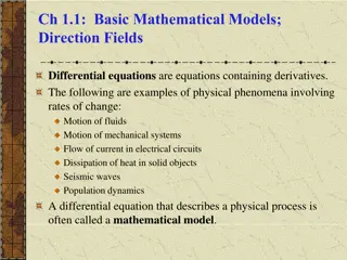
1.3 Differential Equations as Mathematical
Model
Physical meaning of
differentiation:
the variation at certain time or certain place
[Example 1]:
x
(
t
): location,
v
(
t
): velocity,
a
(
t
): acceleration
F
: force,
β
: coefficient of friction,
m
: mass
19
A
: population
人口增加量和人口呈正比
[Example 2]:
人口隨著時間而增加的模型
20
T
:
熱開水溫度
,
T
m
:
環境溫度
t
:
時間
[Example 3]:
開水溫度隨著時間會變冷的模型
21
大一微積分所學的:
的解
Problems
(1)
若等號兩邊都出現
dependent variable
(
如
pages 19, 20
的例
子
)
(2)
若
order of DE
大於
1
(
如
page 18
的例子
)
例如:
該如何解?
Example:
22
Review
•
dependent variable and in
dependent variable
•
DE
•
PDE and ODE
•
Order of DE
•
linear DE and nonlinear DE
•
explicit solution and implicit solution
•
initial value; boundary value
•
IVP
23
Chapter 2 First Order Differential Equation
2-1 Solution Curves without a Solution
Instead of using analytic methods, the DE can be
solved by graphs
(
圖解
)
slopes and the field directions:
x
-axis
y
-axis
(
x
0
, y
0
)
the slope is
f
(
x
0
, y
0
)
24
Example 1
dy
/
dx
= 0.2
xy
From
:
Fig. 2-1-3(a) in “
Differential Equations-with Boundary-Value
Problem”, 9
th
ed., Dennis G. Zill and Michael R. Cullen.
if
y
(0) = 2
y
(0) = -1
if
25
From
:
Fig. 2-1-4 in “
Differential Equations-with Boundary-Value Problem”,
9
th
ed., Dennis G. Zill and Michael R. Cullen.
Example 2
dy
/
dx
= sin(
y
),
y
(0) = –3/2
With initial conditions, one curve can be obtained
26
Advantage:
It can solve some 1
st
order DEs that cannot be solved by
mathematics.
Disadvantage:
It can only be used for the case of the 1st order DE.
It requires a lot of time
27
Section 2-6 A Numerical Method
•
Another way to solve the DE without analytic methods
•
independent variable
x x
0
,
x
1
,
x
2
,
…………
•
Find the solution of
Since approximation
sampling(
取樣
)
前一點的值
取樣間格
28
:
:
:
:
29
Example:
•
dy
(
x
)/
dx
= 0.2
xy
y
(
x
n
+1
) =
y
(
x
n
) + 0.2
x
n
y
(
x
n
)*(
x
n
+1
–
x
n
).
•
dy
/
dx
= sin(
x
)
y
(
x
n
+1
) =
y
(
x
n
) + sin(
x
n
)*(
x
n
+1
–
x
n
).
後頁為
dy
/
dx
= sin(
x
),
y
(0) = –1,
(a)
x
n
+1
–
x
n
= 0.01, (b)
x
n
+1
–
x
n
= 0.1,
(c)
x
n
+1
–
x
n
= 1, (d)
x
n
+1
–
x
n
= 0.1,
dy
/
dx
= 10sin(10
x
)
的例子
Constraint for obtaining accurate results:
(1) small sampling interval (2) small variation of
f
(
x
,
y
)
30
(a)
(b)
(c)
(d)
Blue line: analytic solution;
pink line: numerical solution
31
Advantages
--
It can solve some 1st order DEs that cannot be solved by mathematics.
-- can be used for solving a complicated DE (not constrained for the 1
st
order case)
-- suitable for computer simulation
Disadvantages
-- numerical error (
數值方法
的課程對此有詳細探討
)
32
附錄一
Table of Integration
33
Exercises for Practicing
(not homework, but are encouraged to practice)
1-1: 1, 13, 19, 23, 37
1-2: 3, 13, 21, 33
1-3: 2, 7, 28
2-1: 1, 13, 25, 33
2-6: 1, 3
Explore the world of Differential Equations (DE) with a focus on Boundary Value Problems, guided by Dennis G. Zill and Michael R. Cullen. Dive into the realm of First Order and Higher Order DE, Partial DE, Laplace Transform, Fourier Series, and more. Unravel the complexities of DE through various sections, definitions, notations, and applications outlined in this comprehensive course. Stay organized with the course schedule detailing important dates for homework, midterms, and finals.

Download Presentation

Please find below an Image/Link to download the presentation.
The content on the website is provided AS IS for your information and personal use only. It may not be sold, licensed, or shared on other websites without obtaining consent from the author.If you encounter any issues during the download, it is possible that the publisher has removed the file from their server.
You are allowed to download the files provided on this website for personal or commercial use, subject to the condition that they are used lawfully. All files are the property of their respective owners.
The content on the website is provided AS IS for your information and personal use only. It may not be sold, licensed, or shared on other websites without obtaining consent from the author.
E N D
Presentation Transcript
1 -- Differential Equations (DE) http://djj.ee.ntu.edu.tw/DE.htm ( )
2 3, 4 (AM 10:20~12:10) 205 ( NTUCool) "Differential Equations-with Boundary-Value Problem," Dennis G. Zill and Michael R. Cullen, 9thedition, 2017. (metric version, international version) 15%, 42.5%, 42.5%
3 Office 723 , TEL 33669652 Office hour E-mail: jjding@ntu.edu.tw http://djj.ee.ntu.edu.tw/DE.htm http://disp.ee.ntu.edu.tw/ http://cc.ee.ntu.edu.tw/~tomme/DE/DE.html shengyang@ntu.edu.tw
4 (1) NTUCool (2) http://djj.ee.ntu.edu.tw/DE.htm (3) (4) 40%~90% (5) 11
5 Week Number Date (Wednesday) Remark 1. 9/4 2. 9/11 3. 9/18 4. 9/25: HW1 5. 10/2 6. 10/9 7. 10/16: HW2 8. (Sections 2-2 ~ 4-5) 10/23: Midterms 9. 10/30 10. 11/6 11. 11/13 12. 11/20: HW3 13. 11/27 14. 12/4 15. 12/11: HW4 16. 12/18: Finals (Sections 4-6 ~ 12-4)
6 Introduction (Chap. 1) (Chap. 2) (Chap. 3) First Order DE (Chap. 8 ) (Chap. 4) (Chap. 5 ) Higher Order DE (Sections 4-10, 5-3, ) (Chap. 6) (Sections 12-1, 12-4) (Chapter 12 ) (Chapter 13 ) Partial DE Laplace Transform (Chap. 7 ) Fourier Series (Chap. 11) Transforms Fourier Transform (Chap. 14 )
7 Sections 1-1, 1-2, 1-3 Sections 2-1, 2-2, 2-3, 2-4, 2-5, 2-6 Sections 3-1, 3-2 Sections 4-1, 4-2, 4-3, 4-4, 4-5 Sections 4-6, 4-7 Sections 6-1, 6-2, 6-3, 6-4 Sections 11-1, 11-2, 11-3 Sections 12-1, 12-4 blue colors:
8 Chapter 1 Introduction to Differential Equations 1.1 Definitions and Terminology ( ) (1)Differential Equation (DE): any equation containing derivation (text page 3, definition 1.1) (2) x: independent variable ( ) dy x = 1 y(x): dependent variable dx 3 ( ) d f x dx x ( ) x + = sin( ) ( t f x t dt ) cos 3 0
9 Note: In the text book, f(x) is often simplified as f notations of differentiation 3 4 2 d f dx d f dx d f dx df dx 3 4 2 , , , , . Leibniz notation , , , , . prime notation f f f f (4) , , , , . dot notation f f f f xxx f xxxx f f xf , , , , . subscript notation xx
10 (3) Ordinary Differential Equation (ODE): differentiation with respect to one independent variable 3 2 dx dt dy dt dz dt d u dx d u dx du dx + + = + + + + = 2 xy z cos(6 ) 0 x u 3 2 (4) Partial Differential Equation (PDE): differentiation with respect to two or more independent variables 2 2 u u x t y + = 0 = 2 2 x y
11 (5) Order of a Differentiation Equation: the order of the highest derivative in the equation 7 6 5 4 d u dx d u dx d u dx d u dx 7thorder + + + = 2 2 4 0 7 6 5 4 2 d y dx dy dx 2ndorder + = x 4 5 y e 2
12 (6) Linear Differentiation Equation: ( ) ( ) 1 n n n a x a dx 1 n n d y d dx y dy dx n ( ) ( ) x y ( ) + + + + = x a x a g x 1 0 1 n 1 n dy d dx y d y dx (i) For y, only the terms appear. , ydx , , , 1 n n (ii) All of the coefficient terms am(x) m = 1, 2, , n are independent of y. Property of linear differentiation equations: ( ) ( ) 1 1 n n n n a x a x dx dx 1 2 2 1 1 n n n n a x a x dx dx 1 n n d y d y dy dx dy dx ( ) ( ) x y ( ) + + + + = a x a g x If 1 1 1 1 0 1 1 n n d y d y ( ) ( ) ( ) ( ) x y ( ) x + + + + = a x a g 2 1 0 2 2 and y3= by1+ cy2, then n d y a x d x (if y(x) is treated as the input and g(x) is the output) 1 n d dx y dy d ( ) ( ) x ( ) ( ) x y ( ) x ( ) x + + + + = + a a x a b g c g 3 3 3 1 1 0 3 1 2 n n 1 n n x
13 (7) Non-Linear Differentiation Equation 2 d y dx dy dx + + + = ( 3) 2 y y x 2 2 d y dx dy dx + + = 2 x y e 2 2 d y dx dy dx + + = y x e e 2
[Example 1.1.2] Linear and Nonlinear ODEs (a) The equations 3 d y dx dy dx + = + = + = 3 x ( ) 4 0, " 2 y 0, 5 y x dx xdy y y x x y e 3 are, in turn, linear first-, second-, and third-order ordinary differential equations. We have just demonstrated that the first equation is linear in the variable y by writing it in the alternative form 4xy + y = x. (b) The equations nonlinear term: power not 1 nonlinear term: nonlinear function of y nonlinear term: coefficient depends on y 2 4 x d y dx d y dx ' 2 + = + = + = 2 (1 ) , si n 0, and 0 y y y e y y 2 4 are examples of nonlinear first-, second-, and fourth-order ordinary differential equations, respectively.
15 (8) Explicit Solution (text page 8) The solution is expressed as y = (x) (9) Implicit Solution (text page 8) 2 dy = Example: , dx x 1 + = 2 2 Solution: (implicit solution) 2x y c = 2/ 2 y c x or (explicit solution) 2/ 2 y c x =
16 1.2 Initial Value Problem (IVP) A differentiation equation always has more than one solution. dy dx= 1 for , y = x, y = x+1 , y = x+2 are all the solutions of the above differentiation equation. General form of the solution: y = x+ c, where c is any constant. The initial value ( x = 0) is helpful for obtain the unique solution. dy dx= dy dx= 1 and y(0) = 2 y = x+2 1 and y(2) =3.5 y = x+1.5
17 The kthorder linear differential equation usually requires k independent initial conditions (or k independent boundary conditions) to obtain the unique solution. 2 1 dx d y = 2 solution: y = x2/2 + bx + c, b and c can be any constant (boundary conditions ) y(1) = 2 and y(2) = 3 (initial conditions ) y(0) = 1 and y'(0) =5 (boundary conditions ) y(0) = 1 and y'(3) =2 For the kthorder differential equation, the initial conditions can be 0th~ (k 1)thderivatives at some points.
18 1.3 Differential Equations as Mathematical Model Physical meaning of differentiation: the variation at certain time or certain place ( ) dt ( ) 2 ( ), dt 2 dv t d x t dt dx t ( ) ( ) v t = = [Example 1]: a t = 2 ( ) dt ( ) dx t d x t dt = F v ma = F m 2 x(t): location, v(t): velocity, a(t): acceleration F: force, : coefficient of friction, m: mass
19 [Example 2]: ( ) dt A: population dA t ( ) = kA t
20 [Example 3]: dT dt T: , = ( ) k T T m Tm: t:
21 1 ( ) = + ln dt t c f t dt t ( ) dt dA t ( ) ( ) ( ) = = + f t A t f t dt c ( ) dt ( ) dA t dt dA t 1 t ( ) = + ln A t t c = Example: 1 + 1 + ( ) = = + = ? A t dt c 2 2 4 4 t t Problems (1) dependent variable ( pages 19, 20 ) (2) order of DE 1 ( page 18 )
22 Review dependent variable and independent variable DE PDE and ODE Order of DE linear DE and nonlinear DE explicit solution and implicit solution initial value; boundary value IVP
23 Chapter 2 First Order Differential Equation 2-1 Solution Curves without a Solution Instead of using analytic methods, the DE can be solved by graphs ( ) dy dx= ( ) slopes and the field directions: y-axis , f x y the slope is f(x0, y0) (x0, y0) x-axis
24 Example 1 dy/dx = 0.2xy if y(0) = 2 \\140.112.59.229\ \ \ \ ICON \ Creative Commens 2.5\ icon_by-nc-sa.tiff y(0) = -1 if From Fig. 2-1-3(a) in Differential Equations-with Boundary-Value Problem , 9thed., Dennis G. Zill and Michael R. Cullen.
25 Example 2 dy/dx = sin(y), y(0) = 3/2 \\140.112.59.229\ \ \ \ ICON \ Creative Commens 2.5\ icon_by-nc-sa.tiff From Fig. 2-1-4 in Differential Equations-with Boundary-Value Problem , 9thed., Dennis G. Zill and Michael R. Cullen. With initial conditions, one curve can be obtained
26 Advantage: It can solve some 1storder DEs that cannot be solved by mathematics. Disadvantage: It can only be used for the case of the 1st order DE. It requires a lot of time
27 Section 2-6 A Numerical Method Another way to solve the DE without analytic methods sampling( ) independent variable x x0, x1, x2, ( ) dx dy x ( ) = Find the solution of , f x y ( ) ( ) ( ) dy x y x y x x Since approximation ( f x y dx ) ( ) = = + , 1 n x n , ( ) f x y x n n + 1 n n ( ) ( ) ( )( ) = + , ( ) y x y x f x y x x x + + 1 1 n n n n n n
28 ( ) dx dy x ( ) ( ) ( )( ) ( ) = + , ( ) y x y x f x y x x x = , f x y + + 1 1 n n n n n n If ? ?0 is known ( ) y x ( y x ( ) y x ( ) ( ( ( )( )( )( ) ) ) = + , ( ) y x f x y x x x 1 0 0 0 1 0 ) ( ) y x ( y x = + , ( ) f x y x x x 2 1 1 1 2 1 ) ) = + , ( f x y x x x 3 2 2 2 3 2 : : : :
29 ( ) dx dy x ( ) ( ) ( )( ) ( ) = + , ( ) y x y x f x y x x x = , f x y + + 1 1 n n n n n n Example: dy(x)/dx = 0.2xy y(xn+1) = y(xn) + 0.2xn y(xn)*(xn+1 xn). dy/dx = sin(x) y(xn+1) = y(xn) + sin(xn)*(xn+1 xn). dy/dx = sin(x), y(0) = 1, (a) xn+1 xn= 0.01, (b) xn+1 xn= 0.1, (c) xn+1 xn= 1, (d) xn+1 xn= 0.1, dy/dx = 10sin(10x) Constraint for obtaining accurate results: (1) small sampling interval (2) small variation of f(x, y)
Blue line: analytic solution; pink line: numerical solution 30 (a) (b) 1 1 0.5 0.5 0 0 -0.5 -0.5 -1 -1 \\140.112.59.229\ \ \ \ ICON \ Creative Commens 2.5\ icon_by-nc-sa.tiff \\140.112.59.229\ \ \ \ ICON \ Creative Commens 2.5\ icon_by-nc-sa.tiff -1.5 -1.5 0 5 10 0 5 10 (c) (d) 1 1 0.5 0.5 0 0 -0.5 -0.5 -1 -1 \\140.112.59.229\ \ \ \ ICON \ Creative Commens 2.5\ icon_by-nc-sa.tiff \\140.112.59.229\ \ \ \ ICON \ Creative Commens 2.5\ icon_by-nc-sa.tiff -1.5 -1.5 0 5 10 0 5 10
31 Advantages -- It can solve some 1st order DEs that cannot be solved by mathematics. -- can be used for solving a complicated DE (not constrained for the 1st order case) -- suitable for computer simulation Disadvantages -- numerical error ( )
32 Table of Integration 1/x ln|x| + c cos(x) sin(x) + c sin(x) cos(x) + c tan(x) cot(x) ln|cos(x)| + c ln|sin(x)| + c ax/ln(a) + c ax 1 + 1tan a sin ( / ) x a + 1 c 2 2 x a + 1 x a c 2 2 1/ a x + 1 cos ( / ) x a c 1/ a 2 2 x ax 1 a e + x eax x c a ax 2 a 2 a e x + + 2 x c x2eax 2 a
33 Exercises for Practicing (not homework, but are encouraged to practice) 1-1: 1, 13, 19, 23, 37 1-2: 3, 13, 21, 33 1-3: 2, 7, 28 2-1: 1, 13, 25, 33 2-6: 1, 3