Signal Similarity Measurement and Inner Product Calculation
Learn about the concepts of signal correlation, inner product, and measuring similarity between signals. Explore examples of correlated and uncorrelated signals, as well as how to compute the inner product in MATLAB for signal analysis.

Download Presentation

Please find below an Image/Link to download the presentation.
The content on the website is provided AS IS for your information and personal use only. It may not be sold, licensed, or shared on other websites without obtaining consent from the author. Download presentation by click this link. If you encounter any issues during the download, it is possible that the publisher has removed the file from their server.
E N D
Presentation Transcript
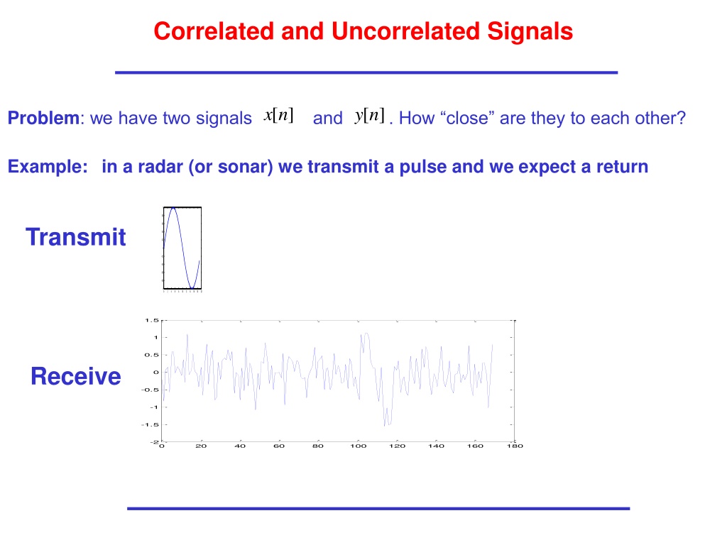
Correlated and Uncorrelated Signals Problem: we have two signals and . How close are they to each other? ] [n x [n y ] Example:in a radar (or sonar) we transmit a pulse and we expect a return 1 0.8 0.6 Transmit 0.4 0.2 0 -0.2 -0.4 -0.6 -0.8 -1 0 2 4 6 8 10 12 14 16 18 20 1.5 1 0.5 Receive 0 -0.5 -1 -1.5 -2 0 20 40 60 80 100 120 140 160 180
Example: Radar Return Since we know what we are looking for, we keep comparing what we receive with what we sent. 1 1 0.8 0.8 0.6 0.6 0.4 0.4 0.2 0.2 0 0 -0.2 -0.2 -0.4 -0.4 -0.6 -0.6 -0.8 -0.8 -1 0 2 4 6 8 10 12 14 16 18 20 -1 0 2 4 6 8 10 12 14 16 18 20 1.5 1 0.5 0 Receive -0.5 -1 -1.5 -2 0 20 40 60 80 100 120 140 160 180 Similar? NO! Think so!
Inner Product between two Signals We need a measure of how close two signals are to each other. This leads to the concepts of Inner Product Correlation Coefficient
Inner Product Problem: we have two signals and . How close are they to each other? ] [n x [n y ] Define: Inner Product between two signals of the same length 1 N = n = * [ ] [ ] r x n y n xy 0 Properties: 1 1 N N = n = n 2 = = * [ ] [ ] [ ] 0 r x n x n x n xx 0 0 2 r r r xy xx yy 2 = [ ] [ ] y n C x n = for some constant C r r r if and only if xy xx yy
How we measure similarity (correlation coefficient) Assume: zero mean Compute: | r | xy = xy r r xx yy Check the value: 0 1 xy 1 0 xy xy x,y uncorrelated x,y strongly correlated
Back to the Example: with no return [n x ] [n y ] [ ] [ ] x n y n 2 3 3 1.5 2 2 1 1 1 0.5 0 0 0 -0.5 -1 -1 -1 -2 -2 -1.5 -3 0 100 200 300 400 500 600 700 800 900 1000 -3 -2 0 100 200 300 400 500 600 700 800 900 0 100 200 300 400 500 600 700 800 900 = . 2 27 r xy = 500 r xx = 982 = r yy . 0 003 NO Correlation! xy
Back to the Example: with return [n x ] 2.5 [ ] [ ] [n y ] x n y n 2 3 1.5 2 2 1 1.5 1 0.5 0 0 1 -0.5 -1 0.5 -1 -1.5 -2 0 -2 0 100 200 300 400 500 600 700 800 900 -3 0 100 200 300 400 500 600 700 800 900 -0.5 0 100 200 300 400 500 600 700 800 900 1000 = 494 r xy = 500 r xx = 754 r yy = 8 . 0 Good Correlation!
Inner Product in Matlab Take two signals of the same length. Each one is a vector: ) ) N = ) 1 ( x ) 2 ( x ( x x N Row vector = ) 1 ( y ) 2 ( y ( y y Row vector Define: Inner Product between two vectors * ) 1 ( y * ) 2 ( y N = n = * ( ) ( ) ) 1 ( x ) 2 ( x x ( ) r x n y n x N xy = 1 * ( ) y N rxy= ' y *y ' x conjugate, transpose
Example Take two signals: y 2.5 3 x 2 2 1.5 1 1 0.5 0 0 -0.5 -1 -1 -1.5 -2 -2 -2.5 -3 0 50 100 150 200 250 300 0 50 100 150 200 250 300 Then: Compute these: = rxy = rxx = ryy 19 7 . = = = * ' 19 7 . x y 0856 . 0 0 xy 218 8 . 241 9 . = * ' 218 8 . x x x,y are not correlated = * ' 241 9 . y y
Example Take two signals: Compute these: 3 x 2 = = * ' 230 9 . rxy x y 1 = = * ' 229 6 . rxx x x 0 -1 = = * ' 234 3 . ryy y y -2 -3 0 50 100 150 200 250 300 Then: y 3 230 9 . 2 = = 9955 . 0 1 xy 1 229 6 . 234 3 . 0 -1 x,y are strongly correlated -2 -3 0 50 100 150 200 250 300
Example Take two signals: y 3 3 x 2 2 1 1 0 0 -1 -1 -2 -2 -3 0 50 100 150 200 250 300 -3 0 50 100 150 200 250 300 Then: Compute these: 230 9 . = = 9955 . 0 1 = = * ' 230 9 . rxy x y xy 229 6 . 234 3 . = = * ' 229 6 . rxx x x x,y are strongly correlated = = * ' 234 3 . ryy y y
Typical Application: Radar Send a Pulse [n s ] n N and receive it back with noise, distortion [n y ] n 0 n 0 n Problem: estimate the time delay , ie detect when we receive it.
Use Inner Product Slide the pulse s[n] over the received signal and see when the inner product is maximum: 1 N = = + * [ ] [ ] [ ] r n y n s [ ] , 0 if rys n n n ys 0 0 n [ ] y 0 n [ s ] N
Use Inner Product Slide the pulse x[n] over the received signal and see when the inner product is maximum: 1 N = n = + = * 0 n [ ] [ ] [ ] r n y n s MAX if ys = 0 = 0 n [ ] y [ s ] N
Matched Filter Take the expression 1 N = + * [ ] [ ] [ ] r n y n s ys = 0 n = ] 1 + ] 1 + + ] 1 + + * * * [ [ ... ] 1 [ [ ] 0 [ [ ] s N y n N s y n s y n Compare this, with the output of the following FIR Filter = + + ] 1 + ] 1 ] 1 + [ r ] ] 0 [ h [ ] ... ] 1 [ h [ [ [ n y n y n h N y n N Then = ] 1 + [n y ] [ r ] [ n r n N [n ] h ys = = * [ ] [ 1 ], ,..., 0 1 h n s N n n N
Matched Filter This Filter is called a Matched Filter [n y ] [ n r ] = ] 1 + [ r ] [ n r n N ys [n ] h = = * [ ] [ 1 ], ,..., 0 1 h n s N n n N + = 1 n N n The output is maximum when 0 = + 1 n n N i.e. 0
Example = [ ], ,..., 0 1 s n n N We transmit the pulse shown below, with length 20 = N 1 0.8 0.6 0.4 [n s ] 0.2 0 -0.2 -0.4 -0.6 -0.8 Max at n=119 119 0 = n -1 0 2 4 6 8 10 12 14 16 18 20 + = 20 1 100 Received signal: 12 [n y ] 1.5 10 [ n r ] 1 [n y ] 8 0.5 6 [n ] 0 h 4 2 -0.5 0 -1 -2 -1.5 -4 -2 0 20 40 60 80 100 120 140 160 180 -6 0 20 40 1 60 80 100 120 140 160 180 200 = = * [ ] [ 1 ], ,..., 0 h n s N n n N
How do we choose a good pulse = [ ], ,..., 0 1 s n n N We transmit the pulse and we receive (ignore the noise for the time being) = [ ] [ ] y n As n 0 n [ n r = ] 1 + ] [ r ] [ n r n N ys [n ] h = = * [ ] [ 1 ], ,..., 0 1 h n s N n n N 1 N where = + * [ ] [ ] [ ] r n A s n n s 0 ys = 0 n = [ ] A r n n 0 ss 1 N = = + * [ ] [ ] [ ] r n s n s The term ss 0 is called the autocorrelation of s[n] . This characterizes the pulse.
Example: a square pulse [n ] rss [n s ] N 1 0 1 N N N n n 1 N = + = * [ ] [ ] [ ] ? r n s n s ss = 0 1 1 N = = N = ] = 2 = = = * ] 0 [ [ ] [ ] [ ] r s s s N ss 0 2 0 2 N N = = + = * ] 1 [ ss 1 [ s ] [ 1 1 r s N See a few values: 0 0 1 1 N k N k 1 = N = = = = + = = * [ ] [ ] [ ] r k s k s N k ss 0 1 0 N = 1 k = + = * [ ] [ ] [ ] 1 r k s k s N k ss 0 k
Compute it in Matlab [n s ] 20 1 18 16 0 1 N n 14 12 10 8 N=20; % data length 6 s=ones(1,N); % square pulse 4 2 rss=xcorr(s); % autocorr 0 -20 -15 -10 -5 0 5 10 15 20 n=-N+1:N-1; % indices for plot stem(n,rss) % plot
Example: Sinusoid 25 1 20 0.8 15 0.6 0.4 10 0.2 0 5 -0.2 -0.4 0 -0.6 -5 -0.8 -1 0 5 10 15 20 25 30 35 40 45 50 -10 -15 -20 = -50 -40 -30 -20 -10 0 10 20 30 40 50 [ ], ,..., 0 49 s n n = [ ], 49 ,..., 49 rss n n
Example: Chirp 30 1 25 0.8 20 0.6 0.4 15 0.2 0 10 -0.2 5 -0.4 -0.6 0 -0.8 -5 -1 0 5 10 15 20 25 30 35 40 45 50 -10 -50 -40 -30 -20 -10 0 10 20 30 40 50 = [ ], ,..., 0 49 s n n = [ ], 49 ,..., 49 rss n n s=chirp(0:49,0,49,0.1)
Example: Pseudo Noise 50 2.5 40 2 1.5 30 1 0.5 20 0 -0.5 10 -1 -1.5 0 -2 -2.5 0 5 10 15 20 25 30 35 40 45 50 -10 -20 -50 -40 -30 -20 -10 0 10 20 30 40 50 = [ ], ,..., 0 49 s n n = [ ], 49 ,..., 49 rss n n s=randn(1,50)
Compare them chirp pseudonoise cos 1 2.5 [n s ] 1 0.8 2 0.8 0.6 1.5 0.6 0.4 1 0.4 0.2 0.2 0.5 0 0 0 -0.2 -0.2 -0.5 -0.4 -0.4 -1 -0.6 -0.6 -1.5 -0.8 -0.8 -2 -1 -1 0 5 10 15 20 25 30 35 40 45 50 0 5 10 15 20 25 30 35 40 45 50 -2.5 0 5 10 15 20 25 30 35 40 45 50 30 50 [n ] rss 25 25 20 40 20 15 30 10 15 20 5 10 0 10 5 -5 0 0 -10 -5 -15 -10 -20 -10 -50 -40 -30 -20 -10 0 10 20 30 40 50 -50 -40 -30 -20 -10 0 10 20 30 40 50 -20 -50 -40 -30 -20 -10 0 10 20 30 40 50 Two best!
Detection with Noise Now see with added noise = + [ ] [ ] [ ] y n As n n w n = ] 1 + + [ r ] [ [ ] n r n n N r n 0 0 ys yw [n ] h = = * [ ] [ 1 ], ,..., 0 1 h n s N n n N
White Noise A first approximation of a disturbance is by White Noise . White noise is such that any two different samples are uncorrelated with each other: 3 [n ] w 2 1 0 -1 -2 -3 -4 0 100 200 300 400 500 600 700 800 900 1000
White Noise The autocorrelation of a white noise signal tends to be a delta function, ie it is always zero, apart from when n=0. [n ] rss n
White Noise and Filters The output of a Filter 1 N = = [ ] [ ] [ ] w n h w n [n ] w 0 [n ] h 1 1 1 1 1 M 1 M M M N N = n = 0 1 n 2 = [ ] [ ] [ ] [ ] [ ] w n h h w n w n 1 2 1 2 = = 0 0 0 2 1 1 1 1 M N N M = 0 1 = n = [ ] [ ] [ ] [ ] h h w n w n 1 2 1 2 = 0 0 2 1 1 1 M N M = = n 2 2 = [ ] [ ] h w n 0 0
White Noise The output of a Filter N = = [ ] [ w ] [ ] w n h n [n ] w 0 [n ] h In other words the Power of the Noise at the ouput is related to the Power of the Noise at the input as 1 N = 2 [ ] P h n P w W = 0 n
Back to the Match Filter = ] 1 + + [ r ] [ [ ] n Ar n n N w n = + [ ] [ ] [ ] y n As n n w n 0 ss 0 [n ] h = = * [ ] [ 1 ], ,..., 0 1 h n s N n n N At the peak: + ] 1 = + + ] 1 [ r ] 0 [ ss [ n N Ar w n N 0 0
Match Filter and SNR At the peak: + ] 1 = + + ] 1 [ r ] 0 [ ss [ n N Ar r n N 0 0 sw 1 1 N N = n = n 2 = 2 2 ] 0 [ ss | [ | ] n | [ | ] n Ar As s 0 0 1 N = 2| ] | [ P s n P W W = 0 n 1 N = 2 [ ] N P s n S = = 0 n SNR N SNR peak 1 N = 2 [ ] s n P W 0 n
Example Transmit a Chirp of length N=50 samples, with SNR=0dB 30 2 25 1.5 20 1 15 0.5 10 0 5 -0.5 0 -1 -5 -10 -1.5 -15 -2 0 200 400 600 800 1000 1200 0 50 Transmitted 100 150 200 250 300 Detected with Matched Filter
Example Transmit a Chirp of length N=100 samples, with SNR=0dB 50 2 40 1.5 30 1 0.5 20 0 10 -0.5 0 -1 -10 -1.5 -2 0 50 100 150 200 250 300 -20 0 200 400 600 800 1000 1200 Detected with Matched Filter Transmitted
Example Transmit a Chirp of length N=300 samples, with SNR=0dB 160 140 2 120 1.5 100 1 80 0.5 60 0 40 -0.5 20 -1 0 -1.5 -20 -2 0 50 100 150 200 250 300 -40 0 200 400 600 800 1000 1200 1400 Transmitted Detected with Matched Filter


")