Seismic Source Parameters in Earthquake Dynamics
1
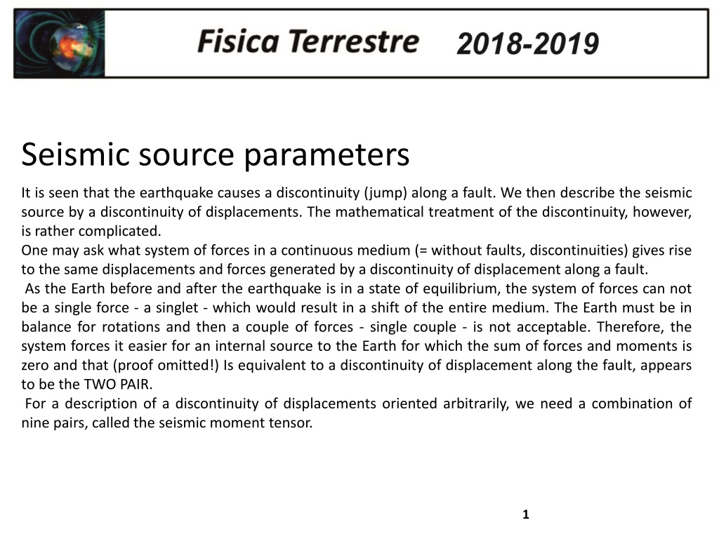
Seismic source parameters
It is seen that the earthquake causes a discontinuity (jump) along a fault. We then describe the seismic
source by a discontinuity of displacements. The mathematical treatment of the discontinuity, however,
is rather complicated.
One may ask what system of forces in a continuous medium (= without faults, discontinuities) gives rise
to the same displacements and forces generated by a discontinuity of displacement along a fault.
As the Earth before and after the earthquake is in a state of equilibrium, the system of forces can not
be a single force - a singlet - which would result in a shift of the entire medium. The Earth must be in
balance for rotations and then a couple of forces - single couple - is not acceptable. Therefore, the
system forces it easier for an internal source to the Earth for which the sum of forces and moments is
zero and that (proof omitted!) Is equivalent to a discontinuity of displacement along the fault, appears
to be the TWO PAIR.
For a description of a discontinuity of displacements oriented arbitrarily, we need a combination of
nine pairs, called the seismic moment tensor.
2
3
Schematic diagram of rupture on a fault that expands from the hypocenter on the fault plane. The motion
starts at the focus and expands according to a front break on the fault plane function of space and time,
separating regions that are in motion by those who still are not. All regions continuously radiate energy
waves P and S. The displacement field varies over the surface of the fault. Note that the direction of
propagation of the rupture is generally not parallel to the direction of sliding
. (Modif. da Bolt, 1988)
4
Simple representation yields seismic waves produced by a complex rupture involving
displacements varying in space and time on irregular fault
First, approximate rupture with a constant average displacement D over a rectangular
fault
Approximate further as a set of force couples.
Approximations are surprisingly successful at matching observed seismograms.
5
Simple representation yields seismic waves
produced by a complex rupture involving
displacements varying in space and time on
irregular fault
First, approximate rupture with a constant
average displacement D over a rectangular fault
Approximate further as a set of force couples.
Approximations are surprisingly successful at
matching observed seismograms.
Terremoto Amatrice 24 agosto 2016
7
The seismic moment is the product of the area of fault surface that ruptures, the average
displacement along that surface, and a constant -- a measure of the elastic property of rock
(i.e. how easily it can be stretched) called the
modulus of rigidity
.
8
The seismic moment is a measure of the size of an earthquake based on the area of fault rupture, the
average amount of
slip
, and the force that was required to overcome the friction sticking the rocks
together that were offset by faulting.
Seismic moment can also be calculated from the amplitude
spectra
of seismic waves.
•
SOURCE SPECTRUM is flat and equal to seismic moment at periods longer than corner frequency 2/T
R
•
Decays below corner frequency
•
Corner frequency shifts to left (lower frequency) for larger earthquakes with longer faults
9
10
The
moment
of an earthquake, is fundamental to our understanding of how dangerous faults of a certain
size can be.
11
A seismic source oriented arbitrarily in space, can be described with the help of the seismic moment
tensor, whose elements are the individual pairs oriented along the spatial axes. With the moment
tensor, you can describe also sources not two pair type, i.e., sources that have an isotropic component
(explosion or implosion).
12
FOR FAULT ORIENTED NORMAL TO COORDINATE AXIS, MOMENT TENSOR IS
Mo is scalar moment
A double couple acting in the plane of the x and y axes (or axis 1 and axis 2) respectively
along the axes x and y, which will be represented by tensor elements with the two pairs
(1,2) and (2,1):
13
The general form of seismic moment tensor is:
The forces equivalent to a generic
point source can be determined
from the analysis of the
eigenvalues and eigenvectors of the
moment tensor.
A common way to decompose the
moment tensor is in terms of
isotropic components, TWO PAIR
(DC) AND LINEAR VECTOR
COMPENSATED DIPOLE (CLVD).
14
15
Complex source model
16
In it is
assigned or determined the displacement
on the fault. According to it determines the seismic
radiation. It 'a relatively easy approach, it is necessary to know only to calculate the Green's functions in
models of the Earth more or less complex (1D, 2D, 3D).
It is widely used in the interpretation of observational data.
Among the kinematic models briefly mention only the model of Haskell for a fault rectangular type (big
earthquakes) and that of Madariaga for a fault of the circular type (earthquakes small-medium).
kinematic source model
Dynamic source model
In them are
assigned or determined stress
and the fall of stress on the fault. According to them it
determines the seismic radiation.
It is a complex problem even in 2D. Analytical solutions exist for semi-infinite fractures.
To solve these problems makes extensive use of computer modeling programs with finite elements, finite
differences, etc.
Are not covered in this course.
17
MODELLO DI HASKELL
18
Modello idealizzato di rottura di Kostrov
(1966) per una rottura che si propaga alla
velocità di rottura v
r
in direzione x. La
frattura inizia quando lo stress all
’
estremità
della rottura supera lo sforzo statico sulla
faglia, τ
S
, e lo stress sulla faglia che scorre si
trova ad un livello costante τ
f
. Lo sforzo
prima della rottura è τ
0
, e lo stress drop è
τ
0
-τ
f
. Ogni punto sulla superficie di rottura
continua lo scorrimento finchè non si ferma
il fronte di rottura e invia un
“
healing
pulse
”
attraverso la faglia.
19
MODELLO DI FRATTURA CIRCOLARE
MADARIAGA
20
I modelli finora discussi non riescono a spiegare le osservazioni neanche nel campo lontano
nel caso di grossi eventi (M≈8) e frequenze basse. Tantomeno riescono a spiegare
la grande
complessità osservata nei segnali ad alta frequenza
(broadband, accelerogrammi) ottenuti
vicino alla sorgente.
La complessità di tali segnali è pertanto da associare alle
condizioni di eterogeneità della
crosta
(lungo la faglia).
La rottura della faglia non è liscia ed uniforme ma variabile ed eterogenea nello spazio.
Porzioni di faglia
che erano sottoposte a grandi sforzi prima del terremoto possono produrre
grossi impulsi di radiazione
, mentre altre parti della faglia offrono una
resistenza molto
grande
in modo da fermare la rottura.
Pertanto alla fine degli anno
’
70 vennero proposti i seguenti modelli per spiegare le
complessità osservate.
21
22
23
24
Momento sismico rilasciato e funzione temporale della
sorgente.
“
L
’
area di faglia
”
mostra una ipotetica storia di
rottura dove il fronte di rottura inizia all
’
ipocentro (stella) ed
attraversa l
’
area di faglia. Le linee tratteggiate indicano il
fronte di rottura in tempi diversi. L
’
area di faglia è
eterogenea, per esempio, ci sono due regioni con alto
momento rilasciato: asperità. Nel plot di M(t), il momento
sismico si accumula fino a raggiungere il valore finale, M
0
, al
tempo T
d
. Le onde dei telesismi sono generate da una
funzione del momento, anche denominata funzione
temporale di sorgente:
L
’
integrale della funzione temporale di sorgente quindi
restituisce il momento sismico complessivo. Si noti che due
asperità risultano in una funzione temporale di due eventi.
Poiché f(t) è una funzione unilaterale, l
’
ampiezza spettrale, la
trasformata di Fourier di f(t) raggiunge il massimo valore a
frequenza zero. Il primo zero spettrale è connesso alla durata
della funzione temporale e l
’
asintoto di decadimento all
’
alta
frequenza è controllato dal momento sismico rilasciato.
25
26
27
Poiché la radiazione delle onde sismiche è controllata dalla velocità di scorrimento ad essa
risulta massima ai bordi della rottura. E
’
il fronte di rottura a produrre radiazioni ad alta
frequenza il resto della faglia irradia le frequenza basse.
28
La faglia è caratterizzata da
sforzi uniformi
lungo la sua estensione. I valori di
sforzo critico
(σ
y
) risultano estremamente variabili. Le regioni ad alta resistenza costituiscono
barriere
(B)
che impediscono la propagazione della rottura.
MODELLO A BARRIERE
(DAS e AKI, 1977)
29
Sforzi
prima
del terremoto
MODELLO A BARRIERE
(DAS e AKI, 1977)
Distribuzione degli
sforzi
dopo
il
terremoto: la faglia è interessata da
una distribuzione di sforzi
eterogenea
30
MODELLO AD ASPERITA
’
(KANAMORI e STEWART, 1978)
Propone uno stato di
sforzi
estremamente variabile sull
’
intera area di faglia. Le zone
sottoposte a sforzo elevato sono le
asperità
che, rompendosi, danno luogo ad un
terremoto complesso. Alla fine della rottura gli sforzi sul piano di faglia sono omogenei.
31
Sforzi
prima
del terremoto
MODELLO AD ASPERITA
’
(KANAMORI e STEWART, 1978)
Sforzi
dopo
la rottura
32
33
34
La distribuzione lungo lo strike dello
scorrimento della superficie di due
terremoti di lunghezza di faglia simile.
(a) Borah Peak, Idaho, 1983: faglia
normale. (b) Imperial Valley, California,
1979: faglia strike-slip. Dati da Sharp et
al. (1982).
The seismic source parameters in earthquake dynamics involve describing a fault as a discontinuity causing displacements, requiring a complex treatment of forces. The Earth's equilibrium necessitates a specific system of forces to explain displacements along faults. The seismic moment tensor, consisting of various force pairs, helps in understanding seismic wave generation. Schematic diagrams illustrate the rupture process on a fault, with energy waves radiating from the hypocenter. The seismic moment quantifies the product of fault area, displacement, and rock elasticity.

Download Presentation

Please find below an Image/Link to download the presentation.
The content on the website is provided AS IS for your information and personal use only. It may not be sold, licensed, or shared on other websites without obtaining consent from the author.If you encounter any issues during the download, it is possible that the publisher has removed the file from their server.
You are allowed to download the files provided on this website for personal or commercial use, subject to the condition that they are used lawfully. All files are the property of their respective owners.
The content on the website is provided AS IS for your information and personal use only. It may not be sold, licensed, or shared on other websites without obtaining consent from the author.
E N D
Presentation Transcript
Seismic source parameters It is seen that the earthquake causes a discontinuity (jump) along a fault. We then describe the seismic source by a discontinuity of displacements. The mathematical treatment of the discontinuity, however, is rather complicated. One may ask what system of forces in a continuous medium (= without faults, discontinuities) gives rise to the same displacements and forces generated by a discontinuity of displacement along a fault. As the Earth before and after the earthquake is in a state of equilibrium, the system of forces can not be a single force - a singlet - which would result in a shift of the entire medium. The Earth must be in balance for rotations and then a couple of forces - single couple - is not acceptable. Therefore, the system forces it easier for an internal source to the Earth for which the sum of forces and moments is zero and that (proof omitted!) Is equivalent to a discontinuity of displacement along the fault, appears to be the TWO PAIR. For a description of a discontinuity of displacements oriented arbitrarily, we need a combination of nine pairs, called the seismic moment tensor. 1
(a) A single force (b) A pair of equal and opposite forces as a tension (c) A pair of equal and opposite forces with time around the z axis (Type I) (d) Two compression are of equal intensity and perpendicular (type II) pairs of forces, tension and (e) Two pair of forces. Their moments around the z axis are equal and opposite (type II) 2
Schematic diagram of rupture on a fault that expands from the hypocenter on the fault plane. The motion starts at the focus and expands according to a front break on the fault plane function of space and time, separating regions that are in motion by those who still are not. All regions continuously radiate energy waves P and S. The displacement field varies over the surface of the fault. Note that the direction of propagation of the rupture is generally not parallel to the direction of sliding. (Modif. da Bolt, 1988) 3
Simple representation yields seismic waves produced by a complex rupture involving displacements varying in space and time on irregular fault First, approximate rupture with a constant average displacement D over a rectangular fault Approximate further as a set of force couples. Approximations are surprisingly successful at matching observed seismograms. 4
Terremoto Amatrice 24 agosto 2016 Rappresentazione 3D del modello di faglia. EVENTO PRINCIPALE
= FL u S = = F S u L Sforzo deformazio ne = M u S 0 The seismic moment is the product of the area of fault surface that ruptures, the average displacement along that surface, and a constant -- a measure of the elastic property of rock (i.e. how easily it can be stretched) called the modulus of rigidity. 7
The seismic moment is a measure of the size of an earthquake based on the area of fault rupture, the average amount of slip, and the force that was required to overcome the friction sticking the rocks together that were offset by faulting. Seismic moment can also be calculated from the amplitude spectra of seismic waves. SOURCE SPECTRUM is flat and equal to seismic moment at periods longer than corner frequency 2/TR Decays below corner frequency Corner frequency shifts to left (lower frequency) for larger earthquakes with longer faults 8
= 3 4 ( / ) 0 M R 0 S 0 0f 9
The moment of an earthquake, is fundamental to our understanding of how dangerous faults of a certain size can be. 10
A seismic source oriented arbitrarily in space, can be described with the help of the seismic moment tensor, whose elements are the individual pairs oriented along the spatial axes. With the moment tensor, you can describe also sources not two pair type, i.e., sources that have an isotropic component (explosion or implosion). 11
A double couple acting in the plane of the x and y axes (or axis 1 and axis 2) respectively along the axes x and y, which will be represented by tensor elements with the two pairs (1,2) and (2,1): = 0 0 0 M 12 0 0 M M 0M Mo is scalar moment 12 0 0 FOR FAULT ORIENTED NORMAL TO COORDINATE AXIS, MOMENT TENSOR IS 12
The general form of seismic moment tensor is: M M M 11 12 13 = M M M M 21 22 23 M M M 31 32 33 The forces equivalent to a generic point source can be determined from the analysis eigenvalues and eigenvectors of the moment tensor. A common way to decompose the moment tensor is in terms of isotropic components, TWO PAIR (DC) AND LINEAR COMPENSATED DIPOLE (CLVD). of the VECTOR 13
EXPLOSION IMPLOSION EARTHQUAKES (DOUBLE COUPLE) OTHER SOURCES (CLVD) 14
Model Source M Couples Focal Mechanism Double-couple (DC) x Strike-slip y z Compensated linear vector dipole (CLVD) x y Ring Fault z x Isotropic Explosion 15
Complex source model kinematic source model In it is assigned or determined the displacement on the fault. According to it determines the seismic radiation. It 'a relatively easy approach, it is necessary to know only to calculate the Green's functions in models of the Earth more or It is widely used in the Among the kinematic models briefly mention only the model of Haskell for a fault rectangular type (big earthquakes) and that of Madariaga for a fault of the circular type (earthquakes small-medium). less complex (1D, observational 2D, 3D). data. interpretation of Dynamic source model In them are assigned or determined stress and the fall of stress on the fault. According to them it determines the seismic radiation. It is a complex problem even in 2D. Analytical solutions exist for semi-infinite fractures. To solve these problems makes extensive use of computer modeling programs with finite elements, finite differences, etc. Are not covered in this course. 16
MODELLO DI HASKELL v = RUPTURE FRONT VELOCITY SLIP STRESS 17
MODELLO DI FRATTURA CIRCOLARE MADARIAGA ( ) ( ) t = = 2 2 . 0 728 u a , ux r t c a r SLIP DISPLACEMENT AND VELOCITY OF P WAVES SLIP STRESS 19
I modelli finora discussi non riescono a spiegare le osservazioni neanche nel campo lontano nel caso di grossi eventi (M 8) e frequenze basse. Tantomeno riescono a spiegare la grande complessit osservata nei segnali ad alta frequenza (broadband, accelerogrammi) ottenuti vicino alla sorgente. La complessit di tali segnali pertanto da associare alle condizioni di eterogeneit della crosta (lungo la faglia). La rottura della faglia non liscia ed uniforme ma variabile ed eterogenea nello spazio. Porzioni di faglia che erano sottoposte a grandi sforzi prima del terremoto possono produrre grossi impulsi di radiazione, mentre altre parti della faglia offrono una resistenza molto grande in modo da fermare la rottura. Pertanto alla fine degli anno 70 vennero proposti i seguenti modelli per spiegare le complessit osservate. 20
Momento sismico rilasciato e funzione temporale della sorgente. L area di faglia mostra una ipotetica storia di rottura dove il fronte di rottura inizia all ipocentro (stella) ed attraversa l area di faglia. Le linee tratteggiate indicano il fronte di rottura in tempi diversi. L area di faglia eterogenea, per esempio, ci sono due regioni con alto momento rilasciato: asperit . Nel plot di M(t), il momento sismico si accumula fino a raggiungere il valore finale, M0, al tempo Td. Le onde dei telesismi sono generate da una funzione del momento, anche denominata funzione temporale di sorgente: ) ( t f = M ( ) t L integrale della funzione temporale di sorgente quindi restituisce il momento sismico complessivo. Si noti che due asperit risultano in una funzione temporale di due eventi. Poich f(t) una funzione unilaterale, l ampiezza spettrale, la trasformata di Fourier di f(t) raggiunge il massimo valore a frequenza zero. Il primo zero spettrale connesso alla durata della funzione temporale e l asintoto di decadimento all alta frequenza controllato dal momento sismico rilasciato. 24
Poich la radiazione delle onde sismiche controllata dalla velocit di scorrimento ad essa risulta massima ai bordi della rottura. E il fronte di rottura a produrre radiazioni ad alta frequenza il resto della faglia irradia le frequenza basse. 27
MODELLO A BARRIERE (DAS e AKI, 1977) La faglia caratterizzata da sforzi uniformi lungo la sua estensione. I valori di sforzo critico ( y) risultano estremamente variabili. Le regioni ad alta resistenza costituiscono barriere (B) che impediscono la propagazione della rottura. 28
MODELLO A BARRIERE (DAS e AKI, 1977) Sforzi prima del terremoto Distribuzione degli sforzi dopo il terremoto: la faglia interessata da una distribuzione eterogenea di sforzi 29
MODELLO AD ASPERITA (KANAMORI e STEWART, 1978) Propone uno stato di sforzi estremamente variabile sull intera area di faglia. Le zone sottoposte a sforzo elevato sono le asperit che, rompendosi, danno luogo ad un terremoto complesso. Alla fine della rottura gli sforzi sul piano di faglia sono omogenei. 30
MODELLO AD ASPERITA (KANAMORI e STEWART, 1978) Sforzi prima del terremoto Sforzi dopo la rottura 31
La distribuzione lungo lo strike dello scorrimento della superficie di due terremoti di lunghezza di faglia simile. (a) Borah Peak, Idaho, 1983: faglia normale. (b) Imperial Valley, California, 1979: faglia strike-slip. Dati da Sharp et al. (1982). 34

 A single force")