Scenarios 2024 Modelling Methodologies


Scenarios
2024 Modelling
Methodologies
TYNDP 2024 Scenarios Strategy
2
2035
The aggregation of national approaches
that reaches EU targets
Deviation from National Trends + scenario
to capture uncertainties and reach EU
targets
Fit-for-55 or
REPowerEU
Overview of 2024 Innovations
3
The innovations implemented in the TYNDP 2024 Scenarios seek to improve those already implemented in
TYNDP 2022
(1)
.
The aim is to enhance the representation of a fast-changing energy system and the integration
of its different
sectors.
The following slides will describe the new methodologies used in the current cycle.
(1)
TYNDP 2022 Scenario Building Guidelines: https://2022.entsos-tyndp-scenarios.eu/building-guidelines/
Overview of 2024 Innovations
4
Tool Chain
for
TYNDP 2024 Scenarios:
-
ETM replacing Ambition Tool
-
DFT replacing TRAPUNTA
Overview of 2024 Innovations
1
Hydrogen Modelling
Hydrogen zones will be modelled
considering a hydrogen market and
production outside the market.
Domestic production of synthetic fuels.
Explicit hydrogen to power modelling.
2
EV Modelling
Improvement of 2022 scenarios.
Transport modelling will include demand
side shifting and Vehicle to grid.
Offshore Modelling
(*)
Modelling of offshore wind hubs.
Hubs include wind farms, electricity grid,
hydrogen pipelines and electrolysers.
Hubs will interconnect with each other and
mainland Europe.
3
4
Heat Modelling
The 2024 Scenario Building process explicitly
considers hybrid heat pumps as heating
technology (boiler and electric heat pump)
that use energy produced by three carriers
(electricity, hydrogen and methane).
5
Expansion Modelling
New approach that enhances run times over
previous cycle, and allows for a larger model
to be run
5
(*)
Only innovation implemented in NT+ Scenario with no expansion. See slide 7.
TYNDP 2024 Deviation Scenarios Topology
6
TYNDP 2024 NT+ Scenario Topology
7
NT+ Scenario uses a simplified methodology compared to Deviation Scenarios because it does not require an expansion and uses directly predefined demand and
capacity figures resulting from TSO data collection.
Hydrogen Modelling
Hydrogen Configurations
9
TYNDP 2022 Scenarios considered 4 different configurations for P2G and H2 grid. However, TYNDP 2024 Scenarios
aggregate them into 2 zones:
-
Zone 1
includes:
-
Direct H2 demand
-
Steel Tank H2 Storages
-
Steam Methane Reformers
-
Shared RES
-
Zone 2
follows the same approach as
Configuration 4 in 2022 Scenarios:
-
Salt Cavern Storages
-
H2 grid
-
Imports (H2 and ammonia)
-
Dedicated RES
Synthetic Fuels
are also explicitly modelled as a new development.
Synthetic Fuels
10
FR00
H2-Z2
Traditional
Supply/Imports
Demand
FR00
Power
€
DE00
H2-Z2
DE00
Power
η
,
€
η
,
€
•
Synthetic fuels are modelled as 1 commodity market within Europe (one single node per fuel type)
•
This node will contain a demand and any country can feed into this node
•
This assumes there are no bottlenecks in the oils and methane pipeline network
CO
2
Supply
H
y
d
r
o
g
e
n
D
e
m
a
n
d
11
ETM quantifies the use of energy across different energy carriers, sectors and applications.
Annual hydrogen demand’s split follows ETM outputs per country. In order to obtain 1 hourly H2 demand profile per country,
the following data is used:
Heating
•
Prosumer: Hydrogen Boilers
using heating normalized profiles from DFT (open power system)
•
Industrial: High Temperature Heating
flat profile
Transport
•
Aviation: Historical kerosene profiles – (Eurostat)
•
Heavy Duty Vehicles: Flat Profile
Industry
•
Final Hydrogen Demand: Flat profile
•
Synthetic fuel production
historical profiles from the industry using the fuel – (Eurostat or Flat)
D
emand Split
12
The hydrogen demand must be split into the 2 Zones.
They will be split by the 4 sectors
•
Feedstock
•
Process heat
•
Prosumer heat
•
Transport
The synthetic fuel production will be assigned to zone 2.
They may be connected to refineries which can be
classed as feedstock. Therefore, the connections to
synthetic fuel will mirror the split for feedstock
Synthetic Fuel
D
e
m
a
n
d
13
E-fuels
•
E-Kerosene
historical
Kerosene profiles
•
E-Diesel
Flat profiles
Synthetic Methane
•
Synthetic fuel producti
o
n
historical
Methane profiles
Explicit hydrogen to power modelling
14
Some countries are expected to have hydrogen-fuelled thermal power plants in the long term.
Electricity/gas TSOs have provided H2 CCGT capacities for target years within the TYNDP data collection.
TYNDP 2024 Scenarios introduce the explicit hydrogen to power modelling, allowing the H2 needed to power CCGTs to
come from the H2 market rather than from a supposedly infinite fuel source (as with other fuels for which no market has been
modelled, e.g. coal):
•
H2 CCGTs in the Electricity Market node are linked to the Hydrogen Market nodes in Plexos.
•
H2 demand will increase proportionally to the fuel offtake of these power plants.
EV Modelling
EV Modelling
TYNDP 2022 Scenarios topology considered an EV Node which was connected to both the Prosumer and the Electricity
Market Nodes. Vehicles were modelled as batteries, being able to charge from the grid to meet the node’s demand (MWh
instead of km) and to feed electricity into the grid (V2G).
TYNDP 2024 Scenarios use the Transport module in PLEXOS: EVs (passenger vehicles) and Charging Stations are explicitly
modelled.
Vehicles will charge at home or in the street depending on the input availability profiles of these stations, and the timing of
charging will be optimized based on costs.
They will also be able to feed electricity into the grid (V2G).
Fast charging is not price driven, so it is not modelled and its electricity profiles are included in the final electricity demand.
16
Electric Vehicle topology
17
Number of EVs connected to Street Charging Station
Number of EVs connected to Street Charging Station
(Availability Profiles)
(Availability Profiles)
Number of EVs connected to
Number of EVs connected to
Prosumer Charging
Prosumer Charging
Station
Station
(Availability Profiles)
(Availability Profiles)
Prosumer EV
Prosumer EV
Street EV
Street EV
Demand (km)
EV
η
=
2
00 wh/km
Charge/Discharge η = 94%
Charge/Discharge η = 94%
Electric Vehicle & Charging Station Properties
18
(i )
https://rem2030.de/rem2030-de/REM-2030-Driving-Profiles.php
(ii)
The availability profile outline the share of vehicles which can be charged by a particular type of charging station.
The share will be split between weekdays/weekends and by station type (Home, Street, Fast)
(iii)
https://platform.elaad.io/analyse/charging/
Electric Vehicle
Electric Vehicle
Charging Stations
Charging Stations
It is important that the values used for modelling EVs in the TYNDP 2024 Scenarios
represent the average European EV owner in the best way.
In 2022 approximately 1.5 million EVs were sold in Europe across multiple models
(1)
.
Most EV models are available in standard and long range, with different sized battery
capacities. Using publicly available data on useable battery capacities of EV models, a
weighted average is calculated for 2030, based on the EVs sold in Europe in 2022
(2)
.
To be in line with the storylines of TYNDP 2024, it is determined that Distributed
Energy will apply the higher ranges of battery capacities of EVs sold in 2022, while
Global Ambition will apply the lower ranges.
It is assumed that technological developments in battery capacities and EV design will
drive an increase in EV battery capacities towards 2050.
Additionally, it is assumed that charging stations at home and by the streets is an
average of what is currently on the market. The methodology on these charging
stations is limited to 22 kW. Higher capacity charging stations are handled separately
in the modelling.
(1)
https://www.jato.com/volkswagen-led-the-european-electric-vehicle-market-in-2022/
(2)
Compare electric vehicles - EV Database (ev-database.org)
Offshore Modelling
Co-optimized offshore energy and infrastructure build-out
SIMPLICITY
ACCURACY
In the TYNDP22 Scenarios all offshore capacity build out was connected radially to their respective home market
TYNDP24 Scenarios will
jointly build out offshore capacity and infrastructure
Capacity and infrastructure will be build out aggregated in so-called "offshore hubs" as a trade-off between simplicity and
accuracy
Offshore hubs represent aggregated PECD areas within the model
20
Offshore Hubs - definition
Offshore Hubs concept
reflects the
combined buildout
of
offshore energy
and
infrastructure
to multiple demand areas
In general, a distinction is made between the
near-shore (<50 km)
and the
far-shore PECD zone (>50 km)
Offshore Bidding Zone
(OBZ) – Individual price area for each hub (aggregated PECD areas) to reduce model complexity
Near shore zone -
Radially connected offshore to
HomeMarket
Exclusion zone
for the nearest 12 nm to account for shoreline protection and reflect the NIMBY effect of coastal communities
21
Offshore Hubs - Assumptions
Interconnector options
will be restricted to
connecting neighbouring Offshore
Hubs (neighbouring aggregated PECD zones) and to related HomeMarket
Hub infrastructure
will be
connected
from
mid-point to mid-point
+ a 30 %
cable routing factor
on top (as in the NSWPH methodology)
The length of the infrastructure to shore will be distance to shoreline +
3
0 km
Hubs and their related home markets can be connected via DC cables as well as
H2 pipelines
Wind offshore capacity within the hubs can be build either connected to the
electricity or H2 grid (via integrated offshore electrolysers). Additionally,
platform-based electrolysers to link the electricity and H2 grid can be build out.
22
Full Topology
23
Offshore technology costs: Bathymetry data
24
Methodology
•
Exclude area till 12 nautical miles
(22.2 km) as customary minimal distance from shore:
ref 1.
(p. 5)
•
Distinguish
between
fixed-bottom
and
floating
technologies
Reasoning:
cost difference
Reference:
Offshore cost elicitation survey
(p. 560)
Differentiating factor: water depth
Fixed-bottom: 0-60m
ref 2.
(p. 7) &
ref 3.
(p. 6)
Floating:
60
m-1000m
ref 4.
(p. 558)
Water depth limit of 1000m
ref 2.
(p. 7) & :
ref 3
.
(p. 4)
Final approach after exchange with WindEurope
Cost
Band 1 (0-200m): Fixed-Bottom & Floating (shallow)
CostBand 2 (200-1000m): Floating (deep)
•
AC to DC
break-even point at
50
km from shore
ref 5.
(p. 5)
Wind Offshore – Investment Candidates
25
Wind Offshore
Fixed AC
Radial
Wind Offshore
Floating AC
Radial
Wind Offshore
Fixed DC
Radial*
Wind Offshore
Floating DC
Radial*
Wind Offshore
Fixed Hub
Wind Offshore
Floating Hub
Wind Offshore
Fixed Hub H2
Wind Offshore
Floating Hub H2
Electrolyzer
Offshore
H2 Pipeline
HVCD Cable
Onshore
HVDC Station
Components
Electrolyzer
Offshore
H2 Pipeline
Includes turbine,
foundation, installation,
array cables
, platform
Cable cost
Mio.€/MW/km
Expansion possible
Compressor costs in
pipeline included
Example E-Hub
* Radial DC connections are only used in special cases, e.g. in Italy
26
AC Electricity Grid
DC Electricity Grid
Electricity and Gas Grid
Hydrogen Pipeline
Exemplary types of offshore wind farms
Hub Structure
Substation
Hub
E-Node
Dedicated
Hub
E-Node Grid
Hub
H
2
-Node
Hub x
Gas station
Inter-Hub H
2
pipelines
Onshore
Zone i
Zone i E-Node
Zone i H
2
-Node
Inter-Hub DC connections
Usage of Bathymetry data in order to differentiate Offshore
technology costs
28
12nm
(22 km)
50 km
HomeMarket
(AC)
OBZ (Hubs)
(
DC)
Hub
(excluded)
Fixed-Bottom
&
Floating (
shallow
)
(0-200m)
Floating (deep)
(200m-1000m)
xx km
HM
Carrier/
Infrastructure
Foundation
type
Zone
Heat Modelling
Heat Demand
ETM provides annual
Flexible Space & Water Heating demand
, which is divided into 2 categories:
-
Prosumer Heating
: To be supplied by Hybrid Heat Pumps (explicitly modelled in PLEXOS for the first time in TYNDP 2024
Scenarios). The electricity/gas that HHP require are a result of the optimization of the model.
-
District Heating
: The electricity/gas that these Heat sources require is given by ETM and integrated into the final
electricity and gas demand profiles (the same approach as TYNDP 2022 Scenarios)
30
Hybrid Heat Pumps Demand
ETM tool provides Heat demand figures for Climate Year 2019.
A methodology has been developed to obtain hourly heat demand hourly profiles per country and for CY 1982-2019:
Based on
Open Power System Data - When To Heat
(1)
demand profiles
•
Data available for all EU27 countries
•
Data available from 2008 to 2020
•
Data from 1982 – 2019 must be calculated
Regression analysis performed to understand the relationship between temperature and heat demand
Model in trained on years 2008 to 2013
Heat demand for all years can be calculated using the trained model
(1)
Data Platform – Open Power System Data (open-power-system-data.org)
31
Climate Data: Linear Regression Analysis
32
Creation of demand timeseries
•
The demand timeseries is split into 2 parts. The first part is Space heating and the
other is water heating.
•
The water heating profiles are not climate dependant and is multiplied by
countries water heating profiles
•
The space heating profile is developed in the following steps
•
The most representative climate year per country is used as the base heating profile.
•
This heating profile is multiplied by the Annual heating demand
•
The heating profiles is then multiplied by the climate variability data in order to give the
climate profiles
33
Hybrid Heat Pumps Modelling
Hybrid Heat Pumps (HHP) combine an electric heat pump with a gas (H2 or CH4) boiler. Each of them will work depending on
the outside temperature (COP curves).
The number of HHP per country and their capacities are given by ETM. However, due to the way they are modelled in
PLEXOS, HHP capacities in the model are equal to the peak heat demand in the node they are connected to.
•
H2 HHP:
-
The electric heat pump is connected to the Prosumer Node
-
The H2 boiler is connected to H2 Zone 2 Node
-
Heat Rate = 0.93 GJ/GJ
•
CH4 HHP:
-
The electric heat pump is connected to the Prosumer Node
-
The CH4 boiler is fuelled with CH4 (non-modelled market)
-
Heat Rate = 0.93 GJ/GJ
34
Coefficient Of Performance
35
Climate and country dependant COP curves are calculated following ETM’s formula:
COP
T
= base COP + COP per degree * T
where
T
is ambient temperature
base COP
= 2.32333
COP per degree
= 0.05783
Expansion Modelling
Expansion Model
37
For a defined electricity and H2 demand, different electricity and H2 systems can be thought of.
PLEXOS has investment loop capabilities from which Scenarios will benefit to define different infrastructure pathways towards a decarbonized
energy system in 2050.
TYNDP 2022 Scenarios used a multi-temporal approach: 25 years were run (2025-2050).
The optimization problem was divided into 8 sub-time horizons of 5 years with a 2-year overlap. However, execution times were too high and
the granularity of the simulation was too low, which meant that batteries could not expand (their behaviour was not visible using this granularity)
TYNDP 2024 introduce a new approach to the multi-temporal expansion. Execution times are significantly reduced and the granularity used
allows the expansion of batteries.
TYNDP 2024 Scenarios cover a 20-year horizon (2030-2050).
A new methodology has been developed to turn those 20 years into 5 and reduce the optimization problems complexity.
Target Years are 2030, 2035, 2040, 2045, 2050, and these are the only years modelled in PLEXOS. However, inputs must ensure that the NPV
of investments in each target year is equivalent to the NPV we would obtain in those years when running the 20-year rolling horizon, so the
build-out in both models is equivalent too.
2024 Expansion Approach
38
Base units
2025-2030
2030-2040
2040-2050
2050-2060
FO&M Charge: OPEX
[€/kW/yr]
Build Cost:
CAPEX
[€/kW]
WACC:
Discount Rate
6%
Economic Life
[yr]
Max Units Built*:
2025-2050
Max Units Built in Year*:
2025-2050
Units built
Each year
Base units
2025-2030
2030-2040
2040-2050
FO&M Charge: OPEX
[€/kW/yr]
Build Cost:
CAPEX
[€/kW]
WACC:
Discount Rate
6%
Economic Life
[yr]
Max Units Built*:
2025-2050
Max Units Built in Year*:
2025-2050
Units built
Each year
= €/kW/5yr
2030-2035
2030-2035
Max Units Built in 5 Years
/5yr
Each 5
years
2030-2031
2031-2032
2032-2033
2033-2034
2034-2035
2035-2036
2022 APPROACH
2024 APPROACH
?%
LT approach – discount rate adjustment
39
Discount rate – 1. Discount factors alignment
The discount
factors are
equalised to those
of the target years
40
Discount rate – 2. NPV alignment
41
Explore the cutting-edge methodologies and tools implemented in the TYNDP 2024 Scenarios to enhance energy system representation and sector integration. Innovations include hydrogen modeling, heat and EV modeling improvements, offshore wind hubs, and deviation scenarios to meet EU targets.

Download Presentation

Please find below an Image/Link to download the presentation.
The content on the website is provided AS IS for your information and personal use only. It may not be sold, licensed, or shared on other websites without obtaining consent from the author. Download presentation by click this link. If you encounter any issues during the download, it is possible that the publisher has removed the file from their server.
E N D
Presentation Transcript
Scenarios 2024 Modelling Methodologies
TYNDP 2024 Scenarios Strategy The aggregation of national approaches that reaches EU targets National Trends+ scenario Increasing range of uncertainty Fit-for-55 or REPowerEU Deviation scenarios 2035 2022 2030 2050 2040 snapshots Deviation from National Trends + scenario to capture uncertainties and reach EU targets 2
Overview of 2024 Innovations The innovations implemented in the TYNDP 2024 Scenarios seek to improve those already implemented in TYNDP 2022(1). The aim is to enhance the representation of a fast-changing energy system and the integration of its different sectors. The following slides will describe the new methodologies used in the current cycle. (1) TYNDP 2022 Scenario Building Guidelines: https://2022.entsos-tyndp-scenarios.eu/building-guidelines/ 3
Overview of 2024 Innovations Tool Chain for TYNDP 2024 Scenarios: - ETM replacing Ambition Tool - DFT replacing TRAPUNTA 4
Overview of 2024 Innovations Hydrogen Modelling Hydrogen zones will be modelled considering a hydrogen market and production outside the market. Domestic production of synthetic fuels. Explicit hydrogen to power modelling. Expansion Modelling New approach that enhances run times over previous cycle, and allows for a larger model to be run Heat Modelling EV Modelling The 2024 Scenario Building process explicitly considers hybrid heat pumps as heating technology (boiler and electric heat pump) that use energy produced by three carriers (electricity, hydrogen and methane). Improvement of 2022 scenarios. Transport modelling will include demand side shifting and Vehicle to grid. Offshore Modelling (*) Modelling of offshore wind hubs. Hubs include wind farms, electricity grid, hydrogen pipelines and electrolysers. Hubs will interconnect with each other and mainland Europe. (*) Only innovation implemented in NT+ Scenario with no expansion. See slide 7. 5
TYNDP 2024 NT+ Scenario Topology NT+ Scenario uses a simplified methodology compared to Deviation Scenarios because it does not require an expansion and uses directly predefined demand and capacity figures resulting from TSO data collection. H2 Node Electricity Node Offshore Wind Hub 7
Breaker slide text Hydrogen Modelling
Hydrogen Configurations TYNDP 2022 Scenarios considered 4 different configurations for P2G and H2 grid. However, TYNDP 2024 Scenarios aggregate them into 2 zones: - Zone 1 includes: - Direct H2 demand - Steel Tank H2 Storages - Steam Methane Reformers - Shared RES - Zone 2 follows the same approach as Configuration 4 in 2022 Scenarios: - Salt Cavern Storages - H2 grid - Imports (H2 and ammonia) - Dedicated RES Synthetic Fuels are also explicitly modelled as a new development. 9
Synthetic Fuels Synthetic fuels are modelled as 1 commodity market within Europe (one single node per fuel type) This node will contain a demand and any country can feed into this node This assumes there are no bottlenecks in the oils and methane pipeline network Traditional Supply/Imports FR00 H2-Z2 DE00 H2-Z2 Demand , , FR00 DE00 CO2 Supply Power Power 10
Hydrogen Demand ETM quantifies the use of energy across different energy carriers, sectors and applications. Annual hydrogen demand s split follows ETM outputs per country. In order to obtain 1 hourly H2 demand profile per country, the following data is used: Heating Prosumer: Hydrogen Boilers using heating normalized profiles from DFT (open power system) Industrial: High Temperature Heating flat profile Transport Aviation: Historical kerosene profiles (Eurostat) Heavy Duty Vehicles: Flat Profile Industry Final Hydrogen Demand: Flat profile Synthetic fuel production historical profiles from the industry using the fuel (Eurostat or Flat) 11
Demand Split The hydrogen demand must be split into the 2 Zones. They will be split by the 4 sectors Feedstock H2 node Sector 2025 2030 2040 2050 Process heat Feedstock 75 60 30 10 Prosumer heat Zone 1 Industry Energetic 50 50 30 15 Transport Transport 75 50 25 15 Feedstock 25 40 70 90 The synthetic fuel production will be assigned to zone 2. Industry Energetic 50 50 70 85 They may be connected to refineries which can be classed as feedstock. Therefore, the connections to synthetic fuel will mirror the split for feedstock Zone 2 Prosumer Heat 100 100 100 100 Transport 25 50 75 85 12
Synthetic Fuel Demand E-fuels E-Kerosene historical Kerosene profiles E-Diesel Flat profiles Synthetic Methane Synthetic fuel production historical Methane profiles 13
Explicit hydrogen to power modelling Some countries are expected to have hydrogen-fuelled thermal power plants in the long term. Electricity/gas TSOs have provided H2 CCGT capacities for target years within the TYNDP data collection. TYNDP 2024 Scenarios introduce the explicit hydrogen to power modelling, allowing the H2 needed to power CCGTs to come from the H2 market rather than from a supposedly infinite fuel source (as with other fuels for which no market has been modelled, e.g. coal): H2 CCGTs in the Electricity Market node are linked to the Hydrogen Market nodes in Plexos. H2 demand will increase proportionally to the fuel offtake of these power plants. CCGT Fuel Offtake H2 Zone 2 Electricity Node Electricity Generation H2 Demand = H2 Demand (input) + CCGT Fuel Offtake 14
Breaker slide text EV Modelling
EV Modelling TYNDP 2022 Scenarios topology considered an EV Node which was connected to both the Prosumer and the Electricity Market Nodes. Vehicles were modelled as batteries, being able to charge from the grid to meet the node s demand (MWh instead of km) and to feed electricity into the grid (V2G). TYNDP 2024 Scenarios use the Transport module in PLEXOS: EVs (passenger vehicles) and Charging Stations are explicitly modelled. Vehicles will charge at home or in the street depending on the input availability profiles of these stations, and the timing of charging will be optimized based on costs. They will also be able to feed electricity into the grid (V2G). Fast charging is not price driven, so it is not modelled and its electricity profiles are included in the final electricity demand. 16
Electric Vehicle topology Electricity Node Prosumer Node Street Charging Station Prosumer Charging Station Charge/Discharge = 94% Charge/Discharge = 94% Street EV Prosumer EV EV = 200 wh/km Number of EVs connected to Street Charging Station (Availability Profiles) Number of EVs connected to Prosumer Charging Station (Availability Profiles) Demand (km) 17
Electric Vehicle & Charging Station Properties Electric Vehicle Parameter Value It is important that the values used for modelling EVs in the TYNDP 2024 Scenarios represent the average European EV owner in the best way. In 2022 approximately 1.5 million EVs were sold in Europe across multiple models (1). Most EV models are available in standard and long range, with different sized battery capacities. Using publicly available data on useable battery capacities of EV models, a weighted average is calculated for 2030, based on the EVs sold in Europe in 2022 (2). To be in line with the storylines of TYNDP 2024, it is determined that Distributed Number of EVs ETM values per country and Target Year 2030 2035 2040 2045 2050 DE Capacity (kWh/Vehicle) 72 83 92 100 60 GA 66 72 81 90 Efficiency (Wh/km) 200 ETM values per country and Target Year converted into hourly profiles based on REM2030(i) Demand (km/Vehicle) Max Charge/Discharge Rate (kW/Vehicle) 7.2 Energy will apply the higher ranges of battery capacities of EVs sold in 2022, while Initial SoC (%) 50 Global Ambition will apply the lower ranges. It is assumed that technological developments in battery capacities and EV design will drive an increase in EV battery capacities towards 2050. Additionally, it is assumed that charging stations at home and by the streets is an average of what is currently on the market. The methodology on these charging stations is limited to 22 kW. Higher capacity charging stations are handled separately in the modelling. Min SoC (%) 20 Availability profiles(ii)based on platform used by ETM (iii) Home Charger Share (%) Availability profiles(ii)based on platform used by ETM (iii) Street Charger Share (%) (i ) https://rem2030.de/rem2030-de/REM-2030-Driving-Profiles.php (ii) The availability profile outline the share of vehicles which can be charged by a particular type of charging station. The share will be split between weekdays/weekends and by station type (Home, Street, Fast) (iii) https://platform.elaad.io/analyse/charging/ Charging Stations Parameter Home Street (1) https://www.jato.com/volkswagen-led-the-european-electric-vehicle-market-in-2022/ MaxCharge/Discharge Rate (kW/Vehicle) 5 16 (2) Compare electric vehicles - EV Database (ev-database.org) Use of SystemCharge( /MWh) 30 35 Charge/DischargeEfficiency (%) 94 94 18
Breaker slide text Offshore Modelling
Co-optimized offshore energy and infrastructure build-out In the TYNDP22 Scenarios all offshore capacity build out was connected radially to their respective home market TYNDP24 Scenarios will jointly build out offshore capacity and infrastructure Capacity and infrastructure will be build out aggregated in so-called "offshore hubs" as a trade-off between simplicity and accuracy Offshore hubs represent aggregated PECD areas within the model SIMPLICITY ACCURACY 20
Offshore Hubs - definition Offshore Hubs concept reflects the combined buildout of offshore energy and infrastructure to multiple demand areas In general, a distinction is made between the near-shore (<50 km) and the far-shore PECD zone (>50 km) Offshore Bidding Zone (OBZ) Individual price area for each hub (aggregated PECD areas) to reduce model complexity Near shore zone - Radially connected offshore to HomeMarket Exclusion zone for the nearest 12 nm to account for shoreline protection and reflect the NIMBY effect of coastal communities 21
Offshore Hubs - Assumptions Interconnector options will be restricted to connecting neighbouring Offshore Hubs (neighbouring aggregated PECD zones) and to related HomeMarket Hub infrastructure will be connected from mid-point to mid-point + a 30 % cable routing factor on top (as in the NSWPH methodology) The length of the infrastructure to shore will be distance to shoreline + 30 km Hubs and their related home markets can be connected via DC cables as well as H2 pipelines Wind offshore capacity within the hubs can be build either connected to the electricity or H2 grid (via integrated offshore electrolysers). Additionally, platform-based electrolysers to link the electricity and H2 grid can be build out. 22
Offshore technology costs: Bathymetry data Methodology Exclude area till 12 nautical miles (22.2 km) as customary minimal distance from shore: ref 1. (p. 5) Distinguish between fixed-bottom and floating technologies Reasoning: cost difference Reference: Offshore cost elicitation survey (p. 560) Differentiating factor: water depth Fixed-bottom: 0-60m ref 2. (p. 7) & ref 3. (p. 6) Floating: 60m-1000m ref 4. (p. 558) Water depth limit of 1000m ref 2. (p. 7) & : ref 3. (p. 4) Final approach after exchange with WindEurope CostBand 1 (0-200m): Fixed-Bottom & Floating (shallow) CostBand 2 (200-1000m): Floating (deep) AC to DC break-even point at 50km from shore ref 5. (p. 5) 24
Wind Offshore Investment Candidates Components Example E-Hub Hub2Hub connection Includes turbine, foundation, installation, array cables, platform HVCD Cable Wind Offshore Fixed Hub Wind Offshore Fixed Hub Wind Offshore Fixed AC Radial Wind Offshore Fixed DC Radial* Wind Offshore Fixed Hub H2 Hub connection to HomeMarket Cable cost Mio. /MW/km Wind Offshore Floating DC Radial* Wind Offshore Floating Hub Wind Offshore Floating AC Radial Wind Offshore Floating Hub H2 HVCD Cable Onshore HVDC Station Expansion possible HVCD Cable H2 Pipeline Electrolyzer Offshore Compressor costs in pipeline included Onshore HVDC Station H2 Pipeline Electrolyzer Offshore * Radial DC connections are only used in special cases, e.g. in Italy 25
Exemplary types of offshore wind farms AC Electricity Grid DC Electricity Grid Electricity and Gas Grid Hydrogen Pipeline 26
Hub Structure Plattform C Plattform B Plattform A Hub x Dedicated P2G Other Plattform CHub x Supply/Demand Gas station Hub Hub E-Node Dedicated H2-Node Zone i H2-Node Plattform BHub x H2-Wind Grid P2G Onshore P2G H2 Power Generation E-Wind Plattform AHub x Hub Zone i E-Node Plattform A E-Node Grid Plattform B Other Plattform C Supply/Demand Substation Inter-Hub H2pipelines Hub z Hub y Inter-Hub DC connections Radial i E-Wind Plattform ARadial iPlattform BRadial iPlattform CRadial i Plattform A Substation Plattform B Plattform C
Usage of Bathymetry data in order to differentiate Offshore technology costs Foundation type Carrier/ Infrastructure Zone xx km E FB Hub OBZ (Hubs) (DC) H2 OBZ (Hubs) (DC) E FL 50 km H2 Offshore HomeMarket (AC) FB HomeMarket (AC) FL 12nm (22 km) 12nm Zone (excluded) (excluded) HM 28
Breaker slide text Heat Modelling
Heat Demand ETM provides annual Flexible Space & Water Heating demand, which is divided into 2 categories: - Prosumer Heating: To be supplied by Hybrid Heat Pumps (explicitly modelled in PLEXOS for the first time in TYNDP 2024 Scenarios). The electricity/gas that HHP require are a result of the optimization of the model. - District Heating: The electricity/gas that these Heat sources require is given by ETM and integrated into the final electricity and gas demand profiles (the same approach as TYNDP 2022 Scenarios) 30
Hybrid Heat Pumps Demand ETM tool provides Heat demand figures for Climate Year 2019. A methodology has been developed to obtain hourly heat demand hourly profiles per country and for CY 1982-2019: Based on Open Power System Data - When To Heat (1) demand profiles Data available for all EU27 countries Data available from 2008 to 2020 Data from 1982 2019 must be calculated Regression analysis performed to understand the relationship between temperature and heat demand Model in trained on years 2008 to 2013 Heat demand for all years can be calculated using the trained model (1) Data Platform Open Power System Data (open-power-system-data.org) 31
Climate Data: Linear Regression Analysis The straight line equation (? = ?? + ?) is used to calculate the heat demand: ???? ?????? = ???? + ? ? = ??????????? ? = ? ????????? ??? = ??????? ?????? ???? HDD = max(?? ??? ??? ?????? ????,0): ????= ??????? ????? ??????????? ?? ??? ??? ??????= ??????????? ?? ? ?? ?????? ?????? Climate variability data: The mean value per hour is calculated over all climates The variance from the mean for each climate year is then calculated in %. 32
Creation of demand timeseries The demand timeseries is split into 2 parts. The first part is Space heating and the other is water heating. The water heating profiles are not climate dependant and is multiplied by countries water heating profiles The space heating profile is developed in the following steps The most representative climate year per country is used as the base heating profile. This heating profile is multiplied by the Annual heating demand The heating profiles is then multiplied by the climate variability data in order to give the climate profiles 33
Hybrid Heat Pumps Modelling Hybrid Heat Pumps (HHP) combine an electric heat pump with a gas (H2 or CH4) boiler. Each of them will work depending on the outside temperature (COP curves). The number of HHP per country and their capacities are given by ETM. However, due to the way they are modelled in PLEXOS, HHP capacities in the model are equal to the peak heat demand in the node they are connected to. H2 HHP: - - The electric heat pump is connected to the Prosumer Node The H2 boiler is connected to H2 Zone 2 Node - Heat Rate = 0.93 GJ/GJ CH4 HHP: - - The electric heat pump is connected to the Prosumer Node The CH4 boiler is fuelled with CH4 (non-modelled market) - Heat Rate = 0.93 GJ/GJ 34
Coefficient Of Performance Climate and country dependant COP curves are calculated following ETM s formula: COPT= base COP + COP per degree * T where T is ambient temperature base COP = 2.32333 COP per degree = 0.05783 35
Breaker slide text Expansion Modelling
Expansion Model For a defined electricity and H2 demand, different electricity and H2 systems can be thought of. PLEXOS has investment loop capabilities from which Scenarios will benefit to define different infrastructure pathways towards a decarbonized energy system in 2050. TYNDP 2022 Scenarios used a multi-temporal approach: 25 years were run (2025-2050). The optimization problem was divided into 8 sub-time horizons of 5 years with a 2-year overlap. However, execution times were too high and the granularity of the simulation was too low, which meant that batteries could not expand (their behaviour was not visible using this granularity) 2025 2026 2027 2028 2029 2030 2031 2032 2033 2034 2035 2036 2037 2038 2039 2040 2041 2042 2043 2044 2045 2046 2047 2048 2049 2050 TYNDP 2024 introduce a new approach to the multi-temporal expansion. Execution times are significantly reduced and the granularity used allows the expansion of batteries. 37
2024 Expansion Approach TYNDP 2024 Scenarios cover a 20-year horizon (2030-2050). A new methodology has been developed to turn those 20 years into 5 and reduce the optimization problems complexity. Target Years are 2030, 2035, 2040, 2045, 2050, and these are the only years modelled in PLEXOS. However, inputs must ensure that the NPV of investments in each target year is equivalent to the NPV we would obtain in those years when running the 20-year rolling horizon, so the build-out in both models is equivalent too. 2030 2035 2040 2045 2050 Target Years 2030 2031 2032 2033 2034 = 2046-2050 = 2030 = 2031-2035 = 2036-2040 = 2041-2045 2022 APPROACH 2024 APPROACH Build Cost: CAPEX [ /kW] Build Cost: CAPEX [ /kW] FO&M Charge: OPEX [ /kW/yr] FO&M Charge: OPEX [ /kW/yr] = /kW/5yr Base units 2025-2030 2030-2040 2040-2050 2050-2060 Base units 2025-2030 2030-2040 2040-2050 2032-2033 2033-2034 2034-2035 2035-2036 WACC: WACC: Units built Each year Units built Each year Each 5 years 2030-2031 2031-2032 Economic Life [yr] Economic Life [yr] /5yr Discount Rate 6% Discount Rate 6% ?% Max Units Built in 5 Years Max Units Built*: 2025-2050 Max Units Built in Year*: 2025-2050 Max Units Built*: 2025-2050 2030-2035 Max Units Built in Year*: 2025-2050 2030-2035 38
LT approach discount rate adjustment Problem: In order to obtain a similar build-out as in the 20-yr model, the discount rate of the 5-yr model objective function needs to be adjusted. In the 20-yr model, the Net Present Value (NPV) calculation follows this expression: 20dfk ??????? NPV20= ?=1 where dfkis the discount factor of year k: 1 dfk= 1+?? with r = discount rate. 4 In the 5-yr model, NPV will be: NPV5= K=1 ??? ???????5 What should be the discount rate R for the 5 years modelling? 2 approaches: 1. Discount factors alignment 2. NPV alignment 39
Discount rate 1. Discount factors alignment Year 20 years model 5 years model Hypothesis 1: All investments are done on every target year (every 5 years). 2030 2031 2032 2033 2034 2035 2036 2037 2038 2039 2040 2041 2042 2043 2044 2045 2046 2047 2048 2049 2050 1.000 0.909 0.826 0.751 0.683 0.621 0.564 0.513 0.467 0.424 0.386 0.350 0.319 0.290 0.263 0.239 0.218 0.198 0.180 0.164 0.149 1.000 0.621 0.386 0.239 0.149 Hypothesis 2: The new discount rate must equalise the discount factor of each target year (2030, 2035, 2040, 2045, 2050). The discount factors are equalised to those of the target years We have: ??5?= ??? (with k = 1 to 5 the years of simulation) 1 1 1 + ?5?= 1 + ?? ? = 1 + ?5 1 (with r and R the discount rates of the 20 and 5 years simulation respectively) For a r = 10%, we get R = 61% 40
Discount rate 2. NPV alignment Hypothesis 1: The investments are made uniformly over a time period. Hypothesis 2: The new discount rate must equalise the NPV of both 20-yr and 5-yr models We have: ???5= ???20 ???????5= 5 Annuity The annuity of a year on the 5-yr model is 5 times the annuity in the 20-yr model. 4 20 5 ??????? 1 + ??= ??????? 1 + ?? ?=1 ?=1 This equation cannot be resolved analytically but it is possible with Excel s solver. For r = 10%, we get R = 47% 41