Scalar Wave Transformation Analysis and Solutions
Scalar wave transformation involving incident waves and orthogonal functions are explored. Derivations, integrations, and coefficient determinations are discussed in detail. Solutions for when x=0 and properties of the scalar functions are also addressed.

Download Presentation

Please find below an Image/Link to download the presentation.
The content on the website is provided AS IS for your information and personal use only. It may not be sold, licensed, or shared on other websites without obtaining consent from the author.If you encounter any issues during the download, it is possible that the publisher has removed the file from their server.
You are allowed to download the files provided on this website for personal or commercial use, subject to the condition that they are used lawfully. All files are the property of their respective owners.
The content on the website is provided AS IS for your information and personal use only. It may not be sold, licensed, or shared on other websites without obtaining consent from the author.
E N D
Presentation Transcript
ECE 6341 Spring 2016 Prof. David R. Jackson ECE Dept. Notes 25 1
Scalar Wave Transformation z Incident wave: ( ) = jkz , , x y z e y This is a scalar function, e.g. the pressure of a sound wave. x = = cos jkz jkr e e Notes: No variation m = 0 Must be finite at the origin (only jn) Must be finite on the z axis (only Pn) = n ( ) ( ) cos n n a j kr P n = 0 Note: Spherical Bessel functions are used here, not Schelkunoff Bessel functions. 2
Scalar Wave Transformation (cont.) (cos )sin P Multiply both sides by and integrate. m Orthogonality: 2 = , n m (cos )sin = + (cos ) P P d 2 0 1 n n m n m 0 ( ) ( ) Harrington Eq. 6.41 Hence 2 ( ) = (cos ) sin cos jkr a j kr e P d m m m + 2 1 m 0 We can now relabel m n. 3
Scalar Wave Transformation (cont.) Let = = = x u kr cos d sin du We then have 1 2 = jxu ( ) ( ) a j x e P u du n n n + 2 1 n + 1 + 1 = jxu ( ) e P u du n 1 4
Scalar Wave Transformation (cont.) The coefficients are therefore determined from + 1 2 = jxu ( ) ( ) a j x e P u du n n n + 2 1 n 1 To find the coefficients, take the limit as x 0. 5
Scalar Wave Transformation (cont.) Recall that x = ( ) ( ) x ( ) x 1 j x J J x ( ) 1/2 + n n + 2 x 2 1 Note: ) 1 n + ( = Therefore, as x 0, we have ! n 1/2 + n x ( ) ~ j x n 1 2 2 x 1/2 + + + n 2 1 n 6
Scalar Wave Transformation (cont.) or n x ( ) ~ j x n 1 2 + + + 1 n 2 1 n As x 0 we therefore have + 1 2 = jxu ( ) ( ) a j x e P u du n n n + 2 1 n 1 + 1 n 2 x = jxu ( ) a e P u du n n + 1 2 2 1 n + + + 1 n 2 1 n 1 7
Scalar Wave Transformation (cont.) Note: If we now let x 0 we get zero on both sides (unless n=0). Solution: Take the derivative with respect to x (n times) before setting x=0. n x ( ) ~ j x n 1 2 + + + 1 n 2 1 n n ! d dx n ( ) ~ j x n 1 2 n + + + 1 n 2 1 n 8
Scalar Wave Transformation (cont.) Hence + 1 2 ( ) 0 ( ) ( ) n = ( ) n n j a ju P u du n n + 2 1 n 1 = + 1 2 ! n ( ) ( ) n n a j u P u du n n + 1 2 2 1 n + + + 1 n 2 1 n 1 1 ( ) ( ) ( ) n = n 2 j u P u du n 0 Define 1 ( ) n I u P u du n n 0 9
Scalar Wave Transformation (cont.) Hence + 2 1 1 2 1 n ( ) n + = + + 1 n 2 2 1 a j I n n n 2 ! n Next, we try to evaluate In: 1 ( ) = n I u P u du n n 0 1 n 1 n d ( ) n = 2 n 1 u u du n 2 ! n du 0 (Rodriguez s formula) 10
Scalar Wave Transformation (cont.) 1 n 1 n d du ( ) n = 2 n 1 I u u du Therefore n n 2 ! n 0 1 1 dg du df du 1 = f du fg g du Integrate by parts n times: 0 0 0 1 1 n ( ) n ( ) n = 2 1 ! 1 I n u du n 2 ! n 0 Notes: m d du n m d du ( ) d du n = 2 = 1 0, = u m n n n ! u n 0, u m n m n m = 1 u = 0 u 11
Scalar Wave Transformation (cont.) or 1 1 2 ( ) n = 2 1 I u du n n 0 Schaum s outline Mathematical Handbook Eq. (15.24): 1 2 ( ) + 1 n 1 ( ) n = 2 1 x dx 1 2 + + 2 1 n 0 12
Scalar Wave Transformation (cont.) Hence 1 2 ( ) + 1 n = I n 1 2 + + + 1 n 2 1 n 13
Scalar Wave Transformation (cont.) We then have 1 2 ( ) + 1 n + 2 1 1 2 1 n ( ) n + = + + 1 n 2 2 1 a j n n 1 2 2 ! n + + + 1 n 2 1 n 1 2 = Note: Hence, )1 1 ( ) ( )( n = + + 1 2 n a j n n ! n 14
Scalar Wave Transformation (cont.) ( ) 1 + = ! n n Now use ( ) ( ) n = + 2 1 n a j n so, Hence n ( ) ( ) ( ) ( ) n = + cos jkz 2 1 e j n j kr P n n = 0 15
Acoustic Scattering z Rigid sphere = 0r a = n a y x Acoustic PW ( ) = pressure of sound wave , , x y z so, 16
Acoustic Scattering (cont.) = i jkz e 2 s = k s = of sound wave = + i s s i = n n r a = 17
Acoustic Scattering (cont.) We have = i ( ) (cos ) a j kr P n n n = 0 n = + n ( ) (2 1) n a j n where Choose = (2) n s ( ) (cos ) b h kr P n n = 0 n Hence, n ( ) j ka = b a (2) n h n n ( ) ka 18
Acoustic Scattering (cont.) Incident wave Real part of pressure scattered by a sphere for ka = 1.0 http://www.paraffinalia.co.uk/Software/examples.shtml 19


")
")
")
")
")
")
")
")
")
")
")
")
")

")
")
")