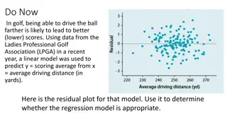
Residual Analysis in Model Selection

Residual analysis is a crucial step in model selection and validation. It involves examining the differences between observed and predicted values, known as residuals, to detect model misspecification, unequal variances, non-normality, outliers, and correlated errors. By utilizing residuals, we can identify potential issues in our models and improve their accuracy. Various examples and visual representations illustrate how residual analysis aids in detecting and addressing these issues in different regression models.

Uploaded on Feb 19, 2025 | 0 Views
Download Presentation

Please find below an Image/Link to download the presentation.
The content on the website is provided AS IS for your information and personal use only. It may not be sold, licensed, or shared on other websites without obtaining consent from the author.If you encounter any issues during the download, it is possible that the publisher has removed the file from their server.
You are allowed to download the files provided on this website for personal or commercial use, subject to the condition that they are used lawfully. All files are the property of their respective owners.
The content on the website is provided AS IS for your information and personal use only. It may not be sold, licensed, or shared on other websites without obtaining consent from the author.
E N D
Presentation Transcript
Residual Analysis Residual Analysis: (1) aid in model selection (2) check assumptions on Best Model: y = 0+ 1x1+ . + kxk+ True error: = ? ( 0+ ???+ .+ ???) In our sample, ? = ? ( ??+ ????+ + ????) ? = y - ? = observed predicted values Residual: Each observation in the data set has a residual value associated with it.
Residual Analysis (continued) ? = y - ? = observed predicted values Residual: Applications: We use the residuals we find from our best model as estimates of the errors to: Detecting Nonzero Error Mean (model Misspecification) 1. 2. Detecting Unequal Variances 3. Detecting Non-Normality 4. Detecting Outliers 5. Detecting Correlated Error
Residual Analysis (continued) 1. Detecting Model Misspecification Violated if non-zero mean (misspecified model) Example: True model is E(y) = 0+ 1x+ 2x2, but we fit y = 0+ 1x + (curvature term omitted) Residual graph: Plot ? vs. Quantitative x s Ideal Plot: Random Scattering of points No pattern usually indicates no problem. If curved indicates quadratics included Not usually a problem when building down Not easy to use this to identify if interactions are needed.
Residual Analysis (continued) Example 12.14 (p. 761) Fit model: E(y) = 0+ 1x y = electrical usage, x = home size Least Squares Linear Regression of USAGE Predictor Variables Coefficient Std Error Constant 903.011 SIZE 0.35594 T P 6.83 0.0000 132.136 0.05477 6.50 0.0000 R Adj R 0.7646 0.7465 Mean Square Error 24102.9 Standard Deviation 155.251 Model statistically useful (p-value = .0000); R-Square is high It is tempting to use this model
Residual Analysis (continued) Example 12.14 (p. 761) Fit model: E(y) = 0+ 1x y = electrical usage, x = home size Residual graph (p. 763): Plot residuals vs. x Scatter Plot of residual vs SIZE 220 Indicates that squared term is omitted! Remedied by adding a squared term to the proposed model. Model results should improve. Linear: R2=.7646; s = 155.25 Quadratics: R2=.9773; s = 50.19 Printout not shown! 130 40 residual -50 -140 -230 1200 2000 2800 3600 SIZE
Residual Analysis (continued) 2. Detecting Unequal Variances (heteroscedasticity) Potential problem when dependent variable( y) is economic data, count-type data, or a proportion Residual graph: Plot ? vs. ? Ideal Plot: Random Scattering of points no pattern usually means no problem (homoscedasticity)
Residual Analysis (continued) Example 12.15 (p. 764) Fit model: E(y) = 0+ 1x y = salary, x = experience (using a dependent variable that is economic in nature) Least Squares Linear Regression of SALARY Predictor Variables Coefficient Constant EXP 2141.38 Std Error 3160.32 160.839 T P 11368.7 3.60 13.31 0.0008 0.0000 R Adj R 0.7869 Mean Square Error 7.469E+07 0.7825 Standard Deviation 8642.44 R2= .78 ; model statistically useful (p-value = 0); It is tempting to use this model.
Statistix software results Residual graph (p. 765): Plot residuals vs. ? Observe funnel pattern Fix this using a variance-stabilizing transformation ( ?, log(y)) Transform the dependent var: y*=log(y) 20000 40000 60000 80000 yhat Scatter Plot of residual vs yhat Unequal Variances! 30000 20000 10000 residual 0 Scatter Plot of residual vs yhat -10000 0.4 -20000 0 0.2 residual 0.0 Be careful with interpretations. -0.2 -0.4 9.8 10.3 10.8 11.3 yhat
Residual Analysis (continued) 3. Detecting Non-normality Graph: Stem-leaf plot of residuals or Zresiduals Look for extreme skewness Mound-shaped usually means no problem Robust slight/moderate departures from normal OK Remedy: Normalizing transformation on y e.g., y* = ?, or y*= log(y)
Residual Analysis (continued) 4. Detecting Outliers data values that are not expected. Have Statistix create Standardized Residual = (y - ?)/s Residual graphs: Stem-leaf plot of std. residuals Plot residuals vs. x Three types of outliers to look for: y-outlier: |std.resid| > 3 Suspect y-outlier: 2 < |std.resid| < 3 x-outlier: x-value vastly different from all others Remedy: Possibly remove outliers from data, but investigate first
Residual Analysis (continued) Handling Outliers what do you do with outliers when they are found? Determine if they were coded correctly or not? 2. Determine if from the correct population. 3. Determine if it is an exceptional observation? 4. Leave it in the analysis. Outliers are a great source of information. Try and determine other variables that may improve the model. 1.
Multicollinearity: Independent variables (x s) are correlated Extrapolation Predictions gone bad Stepwise Regression: Variable-screening method
Multicollinearity (MC) Multicollinearity (Sec. 12.12) x s correlated (MC) Ex 12.18 (p. 775): Federal Trade Commission (FTC) study Predict carbon monoxide content of a cigarette Data collected for 25 cigarettes smoked with a machine y = Carbon monoxide (CO) content (milligrams) x1 = Tar content (milligrams) x2 = Nicotine content (milligrams) x3 = Weight (grams) FTC knows x s have positive relationships with y
Goal of this Example: To recognize the presence of multicollinearity in a multiple linear regression model Model: E(y) = 0+ 1x1+ 2x2 + 3x3 (printout, p. 776) Least Squares Linear Regression of CO Correlations (Pearson) Predictor Variables Coefficient Std Error Constant 3.20219 3.46175 TAR 0.96257 0.24224 NICOTINE -2.63166 3.90056 WEIGHT -0.13048 3.88534 TAR 1.0000 NICOTINE 0.9766 1.0000 WEIGHT 0.4908 0.5002 1.0000 TAR NICOTINE WEIGHT T P VIF 0.0 21.6 21.9 1.3 0.93 3.97 -0.67 -0.03 0.3655 0.0007 0.5072 0.9735 Cases Included 25 Missing Cases 0 R Adj R AICc PRESS 0.9186 0.9070 27.230 89.478 Mean Square Error (MSE) Standard Deviation 2.09012 1.44573 Source Regression 3 Residual 21 Total 24 DF SS MS F 495.258 165.086 78.98 43.893 2.09012 539.150 P 0.0000 Cases Included 25 Missing Cases 0
Multicollinearity (continued) Confusing Printout: Negative betas for Nicotine & Weight Nonsignificant t-tests for Nicotine & Weight Is the FTC wrong? PROBLEM: The x s are moderately to strongly correlated. Multicollinearity exists (inflates standard errors of betas) If not accounted for, leads to erroneous conclusions.
Multicollinearity (continued) Detecting MC: (1) Moderate to high r values for pairs of x s (2) Global F-test significant, all t-tests non-significant (3) betas with opposite signs from theory MC Remedial Measures: (1) Drop 1 or more of highly correlated x s (2) Keep x s, but avoid inferences on betas and restrict predictions to range of sample data
Extrapolation using the model to predict values of x outside the range of the sampled data Example: Interpreting ?0 when the value of x=0 doesn t make sense The same problem exists when we use PI/CIs for values of the x s that fall outside our data set Example: Don t predict the price of a 100,000 mile Mustang if all your collected data are for Mustangs between 10,000 and 75,000 miles Bottom Line be careful when selecting x s to predict for. Make sure that you have collected data that can support the choices.
Stepwise Regression Example: Predict the price of a house Predictors: Size of house, size of lot, number of bedrooms, age of house, condition of house, pool (yes/no), location of house, . Problem: The size of the complete 2nd order model gets too big to be able to use all the variables in the regression analysis. Regression sample size criteria: 10x the number of terms in Model 1
Stepwise Regression (continued) Goal is to reduce the number of independent variables in model building We want to select the most important x s We want to eliminate the least important x s Popular method: Stepwise Regression
Stepwise Regression (continued) Step 1: Fit all possible 1-var models E(y) = 0 + 1xj , select best xj (say, x1) Step 2: Fit all possible 2-var models E(y) = 0 + 1x1 + 2xj , select best xj (say, x2) Step 3: Fit all possible 3-var models E(y) = 0 + 1x1 + 2x2 + 3xj , select best xj Continue until no more significant x s Results look good. Caveats?
Stepwise Regression (continued) Stepwise Regression Problems: (1) Large # of t-tests performed, inflates P(at least 1 Type I error) (2) No higher-order terms in final stepwise model (e.g., curvature, interaction) Recommendation: (1) Use SWR only as a variable screening procedure (2) Use x s selected to begin model building (3) Collect 10x the number of terms in Model 1
Regression Analysis Steps to Follow Step 1:Select independent variables (x's) (Possibly Stepwise regressionif a large # of candidate x s) Step 2:Hypothesize Models Limit # models to control (i.e., don't do too many tests); Include curvature (QN); dummy variables (QL); interaction (QN, QL) Step 3:Fit models to data(using software)
Regression Analysis Steps to Follow Step 4:Model testing (Find "best" model) Global F test, Partial F tests, t-tests Evaluate R2 and 2s Step 5:Residual Analysis (Check assumptions on ) Make model modifications if necessary Step 6:Inferences on Best Model PI for predicting y CI for estimating E(y)


")
")
")
")
")
")

")
")
")
")

")

")
")


")
")

")