Reasoning with Uncertainty: Forms and Challenges
In a world full of uncertainty, mechanisms are needed to reason with unsure, unclear, vague, and ambiguous data. Explore the concepts of monotonicity, the closed world assumption, and non-monotonicity in reasoning, highlighting the challenges they pose in logical reasoning processes.

Download Presentation

Please find below an Image/Link to download the presentation.
The content on the website is provided AS IS for your information and personal use only. It may not be sold, licensed, or shared on other websites without obtaining consent from the author.If you encounter any issues during the download, it is possible that the publisher has removed the file from their server.
You are allowed to download the files provided on this website for personal or commercial use, subject to the condition that they are used lawfully. All files are the property of their respective owners.
The content on the website is provided AS IS for your information and personal use only. It may not be sold, licensed, or shared on other websites without obtaining consent from the author.
E N D
Presentation Transcript
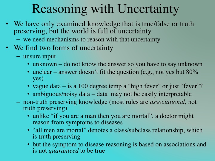
Reasoning with Uncertainty We have only examined knowledge that is true/false or truth preserving, but the world is full of uncertainty we need mechanisms to reason with that uncertainty We find two forms of uncertainty unsure input unknown do not know the answer so you have to say unknown unclear answer doesn t fit the question (e.g., not yes but 80% yes) vague data is a 100 degree temp a high fever or just fever ? ambiguous/noisy data data may not be easily interpretable non-truth preserving knowledge (most rules are associational, not truth preserving) unlike if you are a man then you are mortal , a doctor might reason from symptoms to diseases all men are mortal denotes a class/subclass relationship, which is truth preserving but the symptom to disease reasoning is based on associations and is not guaranteed to be true
Monotonicity Monotonicity starting with a set of axioms, assume we draw certain conclusions if we add new axioms, previous conclusions must remain true the knowledge space can only increase example: assume that person X was murdered and through various axioms about suspects and alibis, we conclude person Y committed the murder later, if we add new evidence, our previous conclusion that Y committed the murder must remain true obviously, the real world doesn t work this way (assume for instance that we find that Y has a valid alibi and Z s alibi was a person who we discovered was lying because of extortion)
The Closed World Assumption In monotonic reasoning, if something is not explicitly known or provable, then it is false this assumption in our reasoning can easily lead to faulty reasoning because its impossible to know everything How can we resolve this problem? we must either introduce all knowledge that is required to solve the problem at the beginning of problem solving or we need another form of reasoning aside from monotonic logic The logic that we have explored so far (first order predicate calculus with chaining or resolution) is monotonic (so is the Prolog system) so now we turn to non-monotonic logics
Non-monotonicity Non-monotonic logic is a logic in which, if new axioms are introduced, previous conclusions can change this requires that we update/modify previous proofs which can be computationally costly We can enhance our previous strategies in logic, add M before a clause M means it is consistent with for all X: bright(X) & student(X) & studies(X,CSC) & M good_economy(time_of_graduation) job(X, time_of_graduation) in a production system, add unless clauses to rules if X is bright, X is a student and X studies computer science, then X will get a job at the time of graduation unless the economy is not good at that time these are forms of assumption-based reasoning
Dependency Directed Backtracking To reduce the computational cost of non-monotonic logic, we need to be able to avoid re-searching the entire search space when a new piece of evidence is introduced otherwise, we have to backtrack to the location where our assumption was introduced and start searching anew from there In dependency directed backtracking, we move to the location of our assumption, make the change and propagate it forward without necessarily having to re-search from that point you have scheduled a meeting on Tuesday at noon because everyone indicated that they were available you cannot find a room, but rather than backtracking to find a new day and time, you just change the day to Thursday
Truth Maintenance Systems In a TMS, inferences are supported by evidence support is directly annotated in the representation so that new evidence can be mapped to conclusions easily if some new piece of evidence is introduced which may overturn a previous conclusion, we need to know if this violates an assumption if so, we negate the assumption and follow through to see what conclusions are no longer true The TMS supports dependency-directed backtracking so that you can easily make changes without having to repeat your search there are several forms of TMS, we will concentrate on the justification TMS (JTMS) but others include assumption-based TMS (ATMS), logic-based TMS (LTMS), and multiple belief reasoners (MBR)
Justification Truth Maintenance System The JTMS is a graph implementation whereby each inference is supported by evidence an inference is supported by items that must be true (labeled as IN items) and those that must be false (labeled as OUT items), things we assume false will be labeled OUT when a new piece of evidence is introduced, we examine the pieces of evidence to see if this either changes it to false or contradicts an assumption, and if so, we change any inferences that were drawn from this evidence to false, and propagate this across the graph
How a JTMS Works The JTMS has three operations inspection through inspection, the JTMS can determine what must be true for a given proposition to be true or what assumptions underlie a proposition modification when new evidence comes to light, modification allows the JTMS to update its beliefs and change its conclusion(s) modification includes the addition or removal of premises, and the addition of new propositions and contradictions to assumptions updating this propagates a modification throughout the entire JTMS by following only those branches impacted It is the updating process in a JTMS that makes it more efficient than a normal backtracker it only backtracks where needed (dependency-directed)
The ABC Murder Mystery Here is an example: a murder has taken place, our suspects are Abbott, Babbitt and Cabot We have the following rules (among others) a person who stands to benefit from a murder is a suspect unless the person has an alibi a person who is an enemy of a murdered person is a suspect unless the person has an alibi an heir stands to benefit from the death of the donor unless the donor is poor a rival stands to benefit from the death of their rival unless the rivalry is not important an alibi is valid if you were out of town at the time unless you have no evidence to support this a picture counts as evidence a signature in a hotel registry is evidence unless it is forged an alibi is valid if someone vouches for you unless that person is a liar
ABC Murder Mystery Continued We know that A is the only heir of the victim and we have no knowledge that the victim was poor We know that B is an enemy of the victim We know that C is a rivalry in business of the victim Currently, we have no evidence of alibis * denotes evidence directly supported by input + denotes IN evidence (must be true) Since we have no evidence of an alibi for any of A, B, C, and because each is a known heir/enemy/rival, we conclude all three are suspects denotes OUT evidence (assumed false)
New Evidence Comes To Light Abbott produces evidence that he was out of town his signature is found in the hotel registry of a respectable hotel in Albany, NY Babbitt s brother-in-law signs an affidavit stating that Babbitt did in fact spend the weekend with him B has an alibi (not in town) and is no longer a suspect We have an alibi for A changing the assumption to true and therefore ruling him out as a suspect Similarly for B, but there is no change made to C, so C remains a suspect
And Finally B s brother-in-law has a criminal record for perjury, so he is a known liar thus, B s alibi is not valid and B again becomes a suspect A friend of C s produces a photograph of C at the meet, shown with the winner the photograph supports C s claim that he was not in town and therefore is a valid alibi, C is no longer a suspect With these final modifications, B becomes our only suspect
Assumption-based TMS (ATMS) The ATMS is the same as a JTMS with two minor changes assumptions can fall into two categories universally accepted as true those that the problem solver is assuming are true but may be retracted (thus, universal assumptions are introduced here) evidence is no longer enumerated as + or -, instead they make up sets of premises Although the latter difference seems irrelevant, it permits the ATMS to entertain multiple belief states at once by changing the assumptions that is, by taking a set of premises and seeing what happens if these assumptions are false there is no single state of the ATMS but instead different subsets of beliefs that can be examined
Example ATMS Dependencies among premises The currently possible belief states (the collection of premises that can be considered true at this at this time)
Abduction In traditional logic, Modus Ponens tell us that if we have A B A we conclude B In abduction, we have instead A B B we conclude A The idea here is that we are saying A can cause B , B happened , we conclude A was its cause this form of reasoning is useful for diagnosis (as an example) but it is not truth-preserving
Using Abductive Reasoning We know that if the battery has lost its charge then the car won t start if the car doesn t start, we can conclude that the battery lost its charge The reason this isn t truth preserving is because there are other possible causes for the car not starting (bad starter, no fuel, bad carburetor, etc) In order to justify our answer, we should examine other causes for the car not starting and disprove those we know there is gas in the car we know the engine is cranking the car was running yesterday etc
How Abduction Can be Truth-Preserving We can still use abduction in a truth-preserving way, but it now takes more work: assume there are several causes for B: A1 B, A2 B, A3 B, A4 B we can rule out A1, A2 and A3 (that is, we introduce ~A1, ~A2, ~A3), therefore we conclude A4 Diagnosis is commonly performed through abduction although in the case of a medical doctor, the possible causes A1, A2, A3, A4 are not ruled out but instead the doctor assigns plausibility values (likelihoods) to each of A1, A2, A3 and A4 how do we get these plausibility values? what if the plausibilities of A1, A2, A3 were all < .5 but A4 was just .5, do we conclude A4?
Set Covering In diagnosis, there may be multiple contributing factors or multiple causes of the symptoms Assume that the following malfunctions (H1-H5, which we will call our hypotheses) can cause the symptoms (observations, O1-O5) as shown H1 O1, O2, O3 H3 O2, O3, O5 H5 O2, O4, O5 O1, O2 and O5 are observed, what is our best explanation? {H1, H4} explains them all but includes O3 (not observed) {H2, H5} explains them all but includes O4 (twice) (not observed) {H1, H3} explains them all but includes O3 (twice) {H1, H4, H5} explains them all but H4 is superfluous Mathematically, this problem is known as set covering abduction is a possible solution to set covering H2 O1, O4 H4 O5
Controlling Abduction Set covering is an NP-complete problem it is computationally expensive because it requires trying all combinations of subsets (of H s) until we have a cover diagnosticians do not perform set covering Some options for set covering/abduction minimal explanation the explanation with the fewest hypotheses parsimonious explanation no superfluous parts highest rated explanation the explanation should contain the most highly evaluated hypotheses (if we evaluate them) these first three combined are known as cost-based abduction consistent explanation the explanation should not include hypotheses that contradict each other this last one is known as coherence-based abduction
Forms of Abduction Aside from trying to build a complete and consistent explanation without superfluous parts, we often want to select the explanation that best explains the data this requires that we somehow gage the hypotheses in terms of their plausibilities How? many different approaches have been taken certainty factors fuzzy logic Dempster Schaeffer, Bayesian forms of reasoning feature based pattern matching neural networks we explore the first four of these in this chapter
Certainty Factors First used in the Mycin system, the idea is that we will attribute a measure of belief to any conclusion that we draw CF(H | E) = MB(H | E) MD(H | E) certainty factor for hypothesis H given evidence E is the measure of belief we have for H minus measure of disbelief we have for H CFs are applied to any hypothesis that we draw by combining CFs of previous hypotheses that are used in the condition portion of the given rule and the CF given to the rule itself To use CFs, we need to annotate every rule with a CF value this comes from the expert ways to combine CFs when we use AND, OR, Combining rules are straightforward: for AND use min for OR use max for NOT, use 1 value (if A is .3, then NOT A is .7) for use * (multiplication)
Assume we have the following rules: A B (.7) A C (.4) D F (.6) B AND G E (.8) C OR F H (.5) We know A, D and G are true (so each have a value of 1.0) B is .7 (A is 1.0, the rule is true at .7, so B is true at 1.0 * .7 = .7) C is .4 F is .6 B AND G is min(.7, 1.0) = .7 (G is 1.0, B is .7) E is .7 * .8 = .56 C OR F is max(.4, .6) = .6 H is .6 * .5 = .30 CF Example
Continued Another combining rule is needed when we can conclude the same hypothesis from two or more rules we already used C OR F H (.5) to conclude H with a CF of .30 let s assume that we also have the rule E H (.5) since E is .56, we have H at .56 * .5 = .28 We now believe H at .30 and at .28, which is true? the two rules both support H, so we want to draw a stronger conclusion in H since we have two independent means of support for H We will use the formula CF1 + CF2 CF1*CF2 CF(H) = .30 + .28 - .30 * .28 = .496 our belief in H has been strengthened through two different chains of logic
CF Advantages and Disadvantages The nice aspects of CFs is that it gives us a mechanism to evaluate hypotheses in order to select the best one(s) for our explanation the formulas are simple to apply experts often think in terms of plausibilities, so getting an expert to supply the CF for a given rule is straight-forward The disadvantages are that CFs are ad hoc (not defined through any formal algebra) no guideline for providing CFs for rules multiple experts may give you inconsistent CFs a single expert may give you less consistent values over time CFs are only provided for rules input is always given the value of 1.0 Many researchers liked the idea of CFs but were not encouraged by the lack of formalism, so other approaches have been developed
Fuzzy Logic Prior to CFs, Zadeh introduced fuzzy logic to introduce shades of grey into logic other logics are two-valued, true or false only Here, any proposition can take on a value in the interval [0, 1] Being a logic, Zadeh introduced the algebra to support logical operators of AND, OR, NOT, X AND Y = min(X, Y) X OR Y = max(X, Y) NOT X = (1 X) X Y = X * Y Where the values of X, Y are determined by where they fall in the interval [0, 1]
Fuzzy Set Theory Fuzzy sets are to normal sets what fuzzy logic is to logic fuzzy set theory is based on fuzzy values from fuzzy logic but includes set operations instead of logic operations The basis for fuzzy sets is defining a fuzzy membership function for a set a fuzzy set is a set of items along with their membership values in the set where the membership value defines how closely that item is to being in that set Example: the set tall might be denoted as tall = { x | f(x) = 1.0 if x > 6 2 , .8 if x > 6 , .6 if x > 5 10 , .4 if x > 5 8 , .2 if x > 5 6 , 0 otherwise} so we can say that a person is tall at .8 if they are 6 1 or we can say that the set of tall people are {Anne/.2, Bill/1.0, Chuck/.6, Fred/.8, Sue/.6}
Fuzzy Membership Function Typically, a membership function is a continuous function (often represented in a graph form like above) given a value y, the membership value for y is u(y), determined by tracing the curve and seeing where it falls on the u(x) axis How do we define a membership function? this is an open question
Using Fuzzy Logic/Sets 1. fuzzify the input(s) using fuzzy membership functions 2. apply fuzzy logic rules to draw conclusions we use the previous rules for AND, OR, NOT, 3. if conclusions are supported by multiple rules, combine the conclusions like CF, we need a combining function, this may be done by computing a center of gravity using calculus 4. defuzzify conclusions to get specific conclusions defuzzification requires translating a numeric value into an actionable item Fuzzy logic is often applied to domains where we can easily derive fuzzy membership functions and have a few rules but not a lot fuzzy logic begins to break down when we have more than a dozen or two rules
Example We have an atmospheric controller which can increase or decrease the temperature of the air and can increase or decrease the fan based on these simple rules if air is warm and dry, decrease the fan and increase the coolant if air is warm and not dry, increase the fan if air is hot and dry, increase the fan and the increase the coolant slightly if air is hot and not dry, increase the fan and coolant if air is cold, turn off the fan and decrease the coolant Our input obviously requires the air temperature and the humidity, the membership function for air temperature is shown to the right if it is 60, it would be considered cold 0, warm 1, hot 0 if it is 85, it would be cold 0, warm .3 and hot .7
Continued Temperature = 85, humidity indicates dry .6 hot .7, warm .3, cold 0, dry .6, not dry .4 (not dry = 1 dry = 1 - .6) Rule 1 has warm and dry warm is .3, dry is .6, so warm and dry = min(.3, .6) = .3 Rule 2 has warm and not dry min(.3, .4) = .3 Rule 3 has hot and dry = min(.7, .3) = .3 our fourth and fifth rules give us 0 since cold is 0 Our conclusions from the first three rules are to decrease the coolant and increase the fan at levels of .3 increase the fan at level of .3 increase the fan at .3 and increase the coolant slightly To combine our results, we might increase the fan by .9 and decrease the coolant (assume increase slightly means increase by ) by .3 - .3/4 = .9/4 Finally, we defuzzify decrease by .9/4 and increase by .9 to actionable amounts
Using Fuzzy Logic The most common applications for fuzzy logic are for controllers devices that, based on input, make minor modifications to their settings for instance air conditioner controller that uses the current temperature, the desired temperature, and the number of open vents to determine how much to turn up or down the blower camera aperture control (up/down, focus, negate a shaky hand) a subway car for braking and acceleration Fuzzy logic has been used for expert systems but the systems tend to perform poorly when more than just a few rules are chained together in our previous example, we just had 5 stand-alone rules when we chain rules, the fuzzy values are multiplied (e.g., .5 from one rule * .3 from another rule * .4 from another rule, our result is .06)
Dempster-Shaeffer Theory The D-S Theory goes beyond CF and Fuzzy Logic by providing us two values to indicate the utility of a hypothesis belief as before, like the CF or fuzzy membership value plausibility adds to our belief by determining if there is any evidence (belief) for opposing the hypothesis We want to know if h is a reasonable hypothesis we have evidence in favor of h giving us a belief of .7 we have no evidence against h, this would imply that the plausibility is greater than the belief p(h) = 1 b(~h) = 1 (since we have no evidence against h, ~h = 0) Consider two hypotheses, h1 and h2 where we have no evidence in favor of either, so b(h1) = b(h2) = .5 we have evidence that suggests ~h2 is less believable than ~h1 so that b(~h2) = .3 and b(~h1) = .5 h1 = [.5, .5] and h2 = [.5, .7] so h2 is more believable
Computing Multiple Beliefs D-S theory gives us a way to compute the belief for any number of subsets of the hypotheses, and modify the beliefs as new evidence is introduced the formula to compute belief (given below) is a bit complex so we present an example to better understand it but the basic idea is this: we have a belief value for how well some piece of evidence supports a group (subset) of hypotheses we introduce a new evidence and multiply the belief from the first with the belief in support of the new evidence for those hypotheses that are in the intersection of the two subsets the denominator is used to normalize the computed beliefs, and is 1 unless the intersection includes some null subsets
Example There are four possible hypotheses for a given patient, cold (C), flu (F), migraine (H), meningitis (M) we introduce a piece of evidence, m1 = fever, which supports {C, F, M} at .6 we also have {Q} (the entire set) with support 1 - .6 = .4 now we add the evidence m2 = nausea which can support {C, F, H} at .7 so that Q = .3 we combine the two sets of beliefs into m3 as follows: Since m3 has no empty sets, the denominator is 1, so the set of values in m3 is already normalized and we do not have to do anything else
Continued When we had m1, we had two sets, {C, F, M} and {Q} When we combined it with m2 (with two sets of its own,{C, F, H} and {Q}), the result was four sets the intersection of {C, F, M} and {C, F, H} = {C, F} the intersection of {C, F, M} and {Q} = {C, F, M} the intersection of {C, F, H} and {Q} = {C, F, H} the intersection of {Q} and {Q} = {Q} We now add evidence m4 = lab culture result that suggest Meningitis, with belief = .8 m4{M} = .8 and m4{Q} = .2 In adding m4, with {M} and {Q}, we intersect these with the four intersected sets above which results in 8 sets shown on the next slide, with some empty sets so our denominator will no longer be 1 and we will have to compute it after computing the numerators
End of Example Sum of empty sets = .336+ .224 = .56, the denominator is 1 - .56 = .44 m5{M} = (.096 + .144) / .44 = .545 m5{ } = (.336 + .224) / .44 = .56 m5{C, F, H} = .056 / .44 = .127 m5{C, F, M} = .036 / .44 = .082 m5{C, F} = .084 / .44 = .191 m5{Q} = .036 / .44 = .055 The most plausible explanation is { } because the evidence tends to contradict (some symptoms indicate Meningitis, another symptom indicates no Meningitis)
Bayesian Probabilities Bayes derived the following formula p(h | E) = p(E | h) * p(h) / sum for all i (p(E | hi) * p(hi)) the probability that h is true given evidence E p(h | E) conditional probability what is the probability that h is true given the evidence E p(E | h) evidential probability what is the probability that evidence E will appear if h is true? p(h) prior probability (or a priori probability) what is the probability that h is true in general without any evidence? the denominator normalizes the conditional probabilities to add up to 1 To solve a problem with Bayesian probabilities we need to accumulate the probabilities for all hypotheses h1, h2, h3 of p(h1 | E), p(h2 | E), p(h3 | E), , p(E | h1), p(E | h2), p(E | h3), and p(h1), p(h2), p(h3), and then its just a straightforward series of calculations
Example The sidewalk is wet, we want to determine the most likely cause it rained overnight (h1) we ran the sprinkler overnight (h2) wet sidewalk (E) Assume the following there was a 50% chance of rain p(h1) = .5 sprinkler is run two nights a week p(h2) = 2/7 = .28 p(wet sidewalk | rain overnight) = .8 p(wet sidewalk | sprinkler) = .9 Now we compute the two conditional probabilities p(h1 | E) = (.5 * .8) / (.5 * .8 + .28 * .9) = .61 p(h2 | E) = (.28 * .9) / (.5 * .8 + .28 * .9) = .39
Independent Events There is a flaw with our previous example if it is likely that it will rain, we will probably not run the sprinkler even if it is the night we usually run it, and if it does not rain, we will probably be more likely to run the sprinkler the next night So we have to be aware of whether events are independent or not two events are independent if P(A & B) = P(A) * P(B) where & means intersect when P(B) <> 0, then P(A) = P(A | B) knowing B is true does not affect the probability of A being true We can also modify our computation by using the formula for conditional independent events P(A & B | C) = P(A | C) * P(B | C) again, & is used to mean intersection we will expand on this shortly
Multiple Pieces of Evidence In our wet sidewalk example, E consisted of one piece of evidence, wet sidewalk what if we have many pieces of evidence? Consider a diagnostic case where there are 10 possible symptoms that we might look for to determine whether a patient has a cold (h1), flu (h2) or sinus infection (h3) E is some subset of {e1, e2, e3, e4, e5, e6, e7, e8, e9, e10} To use Bayes formula, we need to know p(h1), p(h2), p(h3) as well as p(e1 | h1), p(e1 | h2), p(e1 | h3) p(e2 | h1), p(e2 | h2), p(e2 | h3) p(e3 | h1), p(e3 | h2), p(e3 | h3)
Continued But our patient may have several symptoms So we also need p(e1, e2 | h1), p(e1, e2 | h2), p(e1, e2 | h3) p(e1, e3 | h1), p(e1, e3 | h2), p(e1, e3 | h3) p(e2, e3 | h1), p(e2, e3 | h2), p(e2, e3 | h3) p(e1, e2, e3 | h1), p(e1, e2, e3 | h2), p(e1, e2, e3 | h3) How many different probabilities will we need? with 10 pieces of evidence, there are 210 = 1024 different combinations for E, so we will need 3 * 1024 = 3072 evidential probabilities (to go along with the 3 prior probabilities, one for each hypothesis) imagine if E comprised a set of 50 pieces of evidence instead!
Advantages and Disadvantages There two appealing features of probabilities the approach is formal (unlike CFs and unlike the creation of fuzzy membership functions, which are ad hoc) probabilities are easy to compile through statistics p(flu) = number of people who had the flu this year / number of people in the pool p(fever | flu) = number of people with the flu who had a fever / number of people in the pool The primary disadvantages are the need for a great number of probabilities probabilities can be biased for instance, is p(flu) accurate if we gather the data in the summer time rather than in the winter, or year round? the awkwardness if events are not independent (an example follows)
Bayesian Net We can apply the Bayesian formulas for independent and conditionally dependent events in a network form we want to determine the likely cause for seeing orange barrels, flashing lights and bad traffic on the highway two hypotheses: construction, accident (see the figure below) notice T (bad traffic) can be caused by either construction or an accident, orange barrels are only evidence of construction and flashing lights are only evidence of an accident (although it could also be that a driver has been pulled over) construction and accident are not directly related to each other this will help simplify the problem
Computing the Cause We want to compute the cause: construction or accident? first we derive a chain rule to compute a chain of probabilities to handle the dependencies as shown in the figure p(a & b) = p(a | b) * p(b) (again, & means intersection) so p(a & b & c) = p(a) * p(b | a) * p(c | a, b) Therefore, p(C, A, B, T, L) = p(C) * p(A | C) * p(B | C, A) * p(T | B, C, A, B) * p(L | C, A, B, T) with 5 items, we need 25 = 32 probabilities We can reduce p(C, A, B, T, L) to p(C) * p(A) * p(B | C) * p(T | C, A) * p(L, A) because C and A are not linked, p(A | C) = p(A), p(B | C, A) = p(B | C) thus we reduce the total number of terms from 32 to 20 Lets turn to a more complicated problem requiring a slightly different approach
Directed Graph Models We return to the wet sidewalk example but include the season (summer or winter, denoted as hot or cold) the season will impact the probabilities of rain and running the sprinkler our Bayesian network is shown below, notice that unlike the traffic example, we have a cycle (if we remove the directed edges) p(S) prob of the given season p(R | S) prob of rain given the season p(W | S) prob of sprinkler given the season p(WS) prob of a wet sidewalk p(SL | WS) prob of slick sidewalk given it is wet
Continued Notice this network contains a cycle (if we change the links to be undirected, we have a cycle) We cannot apply the chain rule in such a case How do we compute p(WS)? we must remove nodes from the graph to make it acyclic we do this by instantiating various probabilities to either T or F so that we no longer require a specific probability that is leading to the need for the chain rule WS depends on both R and W, so we will generate p(WS) for each of the four values of R and W as shown below we will actually have to do this twice, once for S = hot and once for S = cold x = p(R = t, W = t, S = hot) + p(R = t, W = t, S = cold) we similarly compute the probability p(WS) for each of the other combinations of R and W p(WS) is the sum of these values
Junction Trees The problem with the approach taken in the previous example is having to compute a probability for each combination of nodes that create the cycle what if, instead of R and W, we had 20 nodes that made up the cycle? then we would have to compute 220 combination of probabilities With more forethought in our design, we may be able to avoid this altogether by creating what is known as a junction tree any Bayesian network can be transformed by adding links between the parent nodes of any given node adding links to any cycle of length more than three so that cycles are all of length three or shorter (this helps complete the graph) Each cycle is a clique of no more than 3 nodes each of which forms a junction resulting in dependencies of no more than 3 nodes to restrict the number of probabilities needed
Dynamic Bayesian Networks Cause-effect situations are temporal at time i, an event arises and causes an event at time i+1 the Bayesian belief network is static, it captures a situation at a singular point in time we need a dynamic network instead The dynamic Bayesian network is similar to our previous networks except that each edge represents not merely a dependency, but a temporal change when you take the branch from state i to state i+1, you are not only indicating that state i can cause i+1 but that i was at a time prior to i+1 Here is a state diagram to represents possible utterances for the word tomato Each node represents both a sound and a segment of time


")