Realization of Discrete Time Systems: Structures & Diagrams
Explore the structures and block diagram representations of linear constant-coefficient difference equations in discrete-time systems. Learn about signal flow graphs, IIR systems, FIR systems, and various network structures for implementing these systems effectively.

Download Presentation

Please find below an Image/Link to download the presentation.
The content on the website is provided AS IS for your information and personal use only. It may not be sold, licensed, or shared on other websites without obtaining consent from the author. Download presentation by click this link. If you encounter any issues during the download, it is possible that the publisher has removed the file from their server.
E N D
Presentation Transcript
UNIT-III STRUCTURES FOR THE REALIZATION OF DISCRETE TIME SYSTEMS
Structures for Discrete-Time Systems Block Diagram Representation of Linear Constant-Coefficient Difference Equations Signal Flow Graph Representation of Linear Constant-Coefficient Difference Equations Basic Structures for IIR Systems Transposed Forms Basic Network Structures for FIR Systems Lattice Structures 2
Introduction Example: The system function of a discrete-time system is ) ( 1 az + 1 b b z = , 0 1 H z 1 |z| > |a| Its impulse response will be h[n] = b0anu[n] + b1an-1u[n-1] Its difference equation will be y[n] ay[n-1] = b0x[n] + b1x[n-1] Since this system has an infinite-duration impulse response, it is not possible to implement the system by discrete convolution. However, it can be rewritten in a form that provides the basis for an algorithm for recursive computation. y[n] = ay[n-1] + b0x[n] + b1x[n-1] 3
Block Diagram Representation of Linear Constant-coefficient Difference Equations Multiplication of a sequence by a constant x[n] a ax[n] z-1 Unit delay x[n] x[n-1] + Addition of two sequences x1[n] x1[n] + x2[n] x2[n] 4
Block Diagram Representation of Linear Constant-coefficient Difference Equations M = k b z k ( ) Y z = = ( ) H z 0 = k N ( ) X z k 1 a z k 1 k 1 M = 1 = = k ( ) ( ) ( ) H z H z H z b z 2 1 k N k = k 1 a z 0 k k 1 = ( ) ( ) ( ) V z H z X z 1 = ( ) ( ) ( ) Y z H z V z 2 M = 1 2 = = k ( ) ( ) ( ) H z H z H z b z 1 2 k N = k 1 a z 0 k k 1 k = ( ) ( z ) W ( z ) W z H z X z 2 = ( ) ( ) ( ) Y z H 1 5
Block diagram representation for a general Nth-order difference equation: Direct Form I x[n] b0 v[n] y[n] + + z-1 z-1 b1 a1 + + x[n-1] y[n-1] z-1 z-1 x[n-2] y[n-2] bM-1 aN-1 + + z-1 z-1 bM aN x[n-M] y[n-N] 6
Block diagram representation for a general Nth-order difference equation: Direct Form II b0 x[n] w[n] y[n] + + z-1 z-1 a1 b1 + + w[n-1] w[n-1] z-1 z-1 w[n-2] w[n-2] aN-1 bM-1 + + z-1 z-1 aN bM w[n-N] w[n-M] 7
Combination of delay units (in case N = M) b0 x[n] w[n] y[n] + + z-1 a1 b1 + + z-1 aN-1 bN-1 + + z-1 aN bN 8
Block Diagram Representation of Linear Constant-coefficient Difference Equations 2 An implementation with the minimum number of delay elements is commonly referred to as a canonic form implementation. The direct form I is a direct realization of the difference equation satisfied by the input x[n] and the output y[n], which in turn can be written directly from the system function by inspection. The direct form II or canonic direct form is an rearrangement of the direct form I in order to combine the delay units together. 9
Signal Flow Graph Representation of Linear Constant-coefficient Difference Equations a Attenuator x[n] d e y[n] a z-1 c z-1 Delay Unit b z-1 Node: Adder, Separator, Source, or Sink 10
Basic Structures for IIR Systems Direct Forms Cascade Form Parallel Form Feedback in IIR Systems 11
Basic Structures for IIR Systems Direct Forms N M = k = k = [ ] [ ] [ ] y n a y n k b x n k k k 1 0 M = k k b z k = ( ) H z 0 N = k k 1 a z k 1 12
x[n] y[n] + + z-1 z-1 2 0.75 + + z-1 z-1 -0.125 x[n] y[n] + + z-1 0.75 2 + + + + 1 2 1 2 z z z z-1 = ( ) H z + 1 2 1 . 0 75 . 0 125 z -0.125 16
x[n] y[n] z-1 z-1 2 0.75 z-1 z-1 -0.125 y[n] x[n] z-1 0.75 2 z-1 -0.125 17
Basic Structures for IIR Systems 2 Cascade Form M M 1 2 = N = N k 1 1 1 1 ( ) 1 ( )( 1 ) g z h z h z k k = ( ) H z A 1 1 k k 1 2 = k = k k 1 1 1 1 ( ) 1 ( )( 1 ) c z d z d z k k 1 1 where M = M1+2M2 and N = N1+2N2 . A modular structure that is advantageous for many types of implementations is obtained by combining pairs of real factors and complex conjugate pairs into second-order factors. + a + N 1 2 b b z b z s = k = ( ) 0 1 2 H z k k z k z 1 2 1 a 1 1 2 k k where Ns is the largest integer contained in (N+1)/2. 18
w1[n] y1[n] w2[n] y2[n] w3[n] y3[n] x[n] y[n] b01 b02 b03 z-1 b11 z-1 b12 z-1 b13 a11 a12 a13 z-1 b21 z-1 b22 z-1 b23 a21 a22 a23 + + + + 1 2 1 1 1 2 z 1 ( )( 1 ) z z z z = = ( ) H z + 5 . 0 1 2 1 1 1 . 0 75 . 0 125 1 ( )( 1 . 0 25 ) z z z x[n] y[n] z-1 z-1 z-1 z-1 0.5 0.25 x[n] y[n] z-1 z-1 0.5 0.25 19
Basic Structures for IIR Systems 3 Parallel Form 1 1 N N N 1 ( ) A B e 1 z 1 2 P = k = k = k = + + k ( ) H z C z k k k k k 1 1 1 1 ( )( ) c z d z d z 0 1 1 k k where N = N1+2N2 . If M N, then NP = M - N; otherwise, the first summation in right hand side of equation above is not included. Alternatively, the real poles of H(z) can be grouped in pairs : + z N 1 N e e 1 z S P = k = k = + k ( ) 0 1 H z C z k k k 2 1 a a z 0 1 1 2 k k where NS is the largest integer contained in (N+1)/2, and if NP = M - N is negative, the first sum is not present. 20
C0 w1[n] y1[n] b01 z-1 a11 a21 b11 z-1 x[n] w2[n] y2[n] y[n] b02 b12 z-1 a12 a22 z-1 w3[n] y3[n] b03 b13 z-1 a13 a23 z-1 Parallel form structure for sixth order system (M=N=6). 21
+ + + 1 2 1 1 2 z 7 z 8 + z z z = = + ( ) 8 H z + 1 2 1 2 1 . 0 75 . 0 125 1 . 0 18 75 . 0 125 25 z z = + 8 1 1 1 5 . 0 1 . 0 25 z z 8 y[n] x[n] -7 8 z-1 x[n] y[n] 0.75 8 18 z-1 z-1 0.5 -0.125 -25 z-1 0.25 22
Transposed Forms Transposition (or flow graph reversal) of a flow graph is accomplished by reversing the directions of all branches in the network while keeping the branch transmittances as they were and reversing the roles of the input and output so that source nodes become sink nodes and vice versa. y[n] y[n] x[n] x[n] z-1 z-1 a a x[n] y[n] z-1 a 23
x[n] y[n] b0 z-1 z-1 b1 a1 z-1 z-1 b2 a2 bN-1 aN-1 z-1 z-1 bN aN x[n] y[n] b0 z-1 z-1 a1 b1 z-1 z-1 a2 b2 aN-1 bN-1 z-1 z-1 aN bN 24
x[n] y[n] b0 z-1 a1 b1 z-1 a2 b2 aN-1 bN-1 x[n] y[n] z-1 b0 aN bN z-1 b1 a1 z-1 b2 a2 bN-1 aN-1 z-1 bN aN 25
Basic Network Structures for FIR Systems Direct Form It is also referred to as a tapped delay line structure or a transversal filter structure. Transposed Form Cascade Form = n 0 M M S = k = = + + 1 2 n ( ) [ ] ( ) H z h n z b b z b z 0 1 2 k k k 1 where MS is the largest integer contained in (M + 1)/2. If M is odd, one of coefficients b2k will be zero. 26
Direct Form For causal FIR system, the system function has only zeros (except for poles at z = 0) with the difference equation: y[n] = SMk=0 bkx[n-k] It can be interpreted as the discrete convolution of x[n] with the impulse response h[n] = bn, n = 0, 1, , M, 0 , otherwise. 27
Direct Form (Tapped Delay Line or Transversal Filter) x[n] y[n] b0 z-1 b1 z-1 b2 bN-1 z-1 bN x[n] z-1 z-1 z-1 h[0] h[1] h[2] h[M-1] h[M] y[n] 28
Transposed Form of FIR Network y[n] z-1 z-1 z-1 z-1 h[M] h[M-1] h[M-2] h[2] h[1] h[0] x[n] 29
Cascade Form Structure of a FIR System x[n] y[n] b01 b02 b0Ms z-1 z-1 z-1 b11 b12 b1Ms z-1 z-1 z-1 b21 b22 b2Ms 30
Structures for Linear-Phase FIR Systems Structures for Linear Phase FIR Systems : h[M-n] = h[n] for n = 0, 1, ..., M For M is an even integer : Type I y[n] = Sk=0(M/2)-1 h[k](x[n-k] + x[n-M+k]) + h[M/2]x[n-M/2] For M is an odd integer : Type II y[n] = Sk=0(M-1)/2 h[k](x[n-k] + x[n-M+k]) h[M-n] = -h[n] for n = 0, 1, ..., M For M is an even integer : Type III y[n] = Sk=0(M/2)-1 h[k](x[n-k] - x[n-M+k]) For M is an odd integer : Type IV y[n] = Sk=0(M-1)/2 h[k](x[n-k] - x[n-M+k]) 31
Direct form structure for an FIR linear-phase when M is even. x[n] z-1 z-1 z-1 z-1 z-1 z-1 h[0] h[1] h[2] h[(M/2)-1] h[M/2] y[n] Direct form structure for an FIR linear-phase when M is odd. x[n] z-1 z-1 z-1 z-1 z-1 z-1 z-1 h[0] h[1] h[2] h[(M-3)/2] h[(M-1)/2] y[n] 32
Lattice Structures Theory of autoregressive signal modeling : Lattice Structure Development of digital filter structures that are analogous to analog filter structures : Wave Digital Filters Another structure development approach is based on state-variable representations and linear transformations. 33
Lattice Structures 2 FIR Lattice 1 N ( ) Y z = m = = = m ( ) ( ) H z A z a mz ( ) X z 1 The coefficients {ki} in the lattice structures are referred to as the k-parameters, which are called reflection coefficients or PARCOR coefficients. When used in signal modeling, the k-parameters are estimated from a data signal . Given a set of k-parameters, the system function can be found and therefore the impulse response : by recurrence formula for computing A(z) in terms of the intermediate system functions 34
Reflection coefficients or PARCOR coefficients structure x[n] e0[n] e1[n] e2[n] eN-1[n] eN[n] y[n] -k1 -k2 -kN -kN -k1 -k2 z-1 z-1 z-1 e~0[n] e~1[n] e~2[n] e~N-1[n] e~N[n] Signal flow graph of an FIR lattice system e0[n] = e~0[n] = x[n] ei[n] = ei-1[n] kie~i-1[n-1], i = 1, 2, , N, e~i[n] = -kiei-1[n] + e~i-1[n-1] y[n] = eN[n] 35
A recurrence formula for computing A(z) = H(z) = Y(z)/X(z) can be obtained in terms of intermediate system functions: 1 i ( ) E z = m = = ( ) i m ( ) A z a z i i m ( ) E z 1 O By recursive technique: ai(i) = ki , am(i) = am(i-1) - ki ai-m(i-1) , m = 1, 2, ..., (i-1) Or by reverse recursive technique: ki = ai(i) am(i-1) = [am(i) + kiai-m(i)]/[1 ki2], m = 1, 2, , (i 1) 36
Example: = (1-0.8jz-1)(1+0.8jz-1)(1-0.9z-1) = 1 0.9z-1 + 0.64z-2 0.576z-3. a1(3) = 0.9, a2(3) = -0.64, and a3(3) = 0.576 A(z) Then, The k-parameter can be computed as follow: k3 = a3(3) = 0.576 a1(2) = [a1(3) + k3a2(3)]/[1 k32] = 0.79518245 a2(2) = [a2(3) + k3a1(3)]/[1 k32] = - 0.18197491 k2 = a2(2) = - 0.18197491 a1(1) = [a1(2) + k2a1(2)]/[1 k22] = 0.67275747 k1 = a1(1) = 0.67275747 37
x[n] y[n] -0.6728 +0.182 -0.576 -0.576 -0.6728 +0.182 z-1 z-1 z-1 z 1 z 1 z-1 x[n] -0.9 0.64 -0.576 y[n] 38
All-Pole Lattice A lattice system with an all-pole system function H(z) = 1/A(z) can be developed from the FIR lattice . all roots of A(z) must be inside the unit circle: |ki| < 1, i = 1, ..., N ei[n] ei-1[n] eN[n] = x[n] Ei-1[n] = ei[n] + kie~i-1[n-1], i = N, (N-1), 1, e~i[n] = -kiei-1[n] + e~i-1[n-1] y[n] = e0[n] = e~0[n] ki z-1-ki z-1 e~i[n] e~i-1[n] x[n] e0[n] e1[n] e2[n] eN-1[n] eN[n] y[n] kN kN-2 k1 -k1 -kN -kN-2 z-1 z-1 z-1 e~N[n] e~N-1[n] e~1[n] e~0[n] 39
Basic all-pole lattice structures Three-multiplier form Four-multiplier, normalized form N = cos i = ( ) H z 1 i ( ) A z Four-multiplier, Kelly-Lochbaum form : was first derived as an acoustic tube model for speech synthesis. N = + 1 ( ) k i = ( ) H z 1 i ( ) A z 40
ei[n] ei-1[n] -ki ki Three-multiplier form e i[n] (1 - ki2) e i-1[n] ei[n] cos qi ei-1[n] -sin qi sin qi Four-multiplier, normalized form e i[n] cos qi e i-1[n] ei[n] (1 + ki) ei-1[n] -ki ki Four-multiplier, Kelly- Lochbaum form e i[n] (1 - ki) e i-1[n] 41
Lattice Systems with Poles and Zeros 1 i N ( ) ( ) ( ) Y z c z A ( z ) B z = i = = = ( ) H z i i ( ) ( ) X z A z A z 0 N = m = m ( ) B z b z m 0 N = m = ( ) i b c c 1 a m m i i m + i x[n] = eN[n] eN-1[n] eN-2[n] e1[n] e0[n] Section N Section N - 1 Section 1 e N[n] e N-1[n] e N-2[n] e 1[n] e 0[n] cN cN-1 cN-2 c1 c0 y[n] 42
Example of lattice IIR filter with poles and zeros x[n] y[n] z-1 3 0.9 z-1 3 -0.64 z-1 0.576 x[n] 0.576 -0.182 0.6728 -0.576 0.182 -0.6728 z-1 z-1 z-1 3.9 5.4612 4.5404 y[n] 43


")


")
")


")


 = H(z) = Y(z)/X(z)")