Read Mapping in Genomics
Read mapping is a critical process in genomics that involves aligning sequencing reads to a reference genome or transcriptome. By detecting similarities between reads and potential targets, mapping helps identify the specific chromosome, gene, and position that a read corresponds to. This process relies on achieving set similarity thresholds, akin to tools like BLAST, to accurately pinpoint the location of a read on the reference sequence.

Download Presentation

Please find below an Image/Link to download the presentation.
The content on the website is provided AS IS for your information and personal use only. It may not be sold, licensed, or shared on other websites without obtaining consent from the author.If you encounter any issues during the download, it is possible that the publisher has removed the file from their server.
You are allowed to download the files provided on this website for personal or commercial use, subject to the condition that they are used lawfully. All files are the property of their respective owners.
The content on the website is provided AS IS for your information and personal use only. It may not be sold, licensed, or shared on other websites without obtaining consent from the author.
E N D
Presentation Transcript
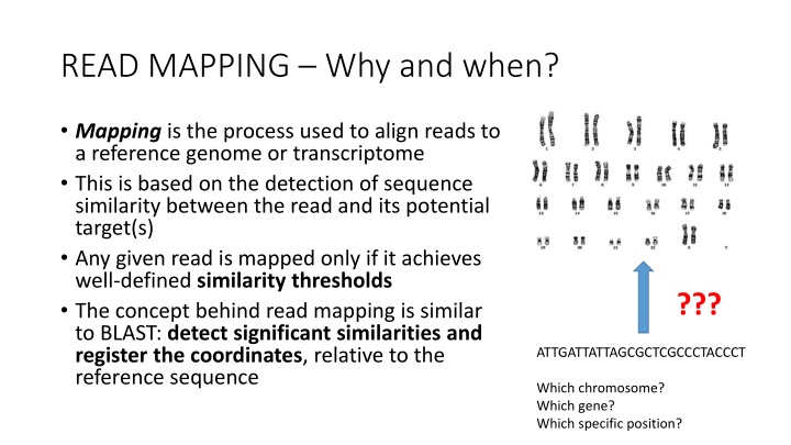
READ MAPPING Why and when? Mapping is the process used to align reads to a reference genome or transcriptome This is based on the detection of sequence similarity between the read and its potential target(s) Any given read is mapped only if it achieves well-defined similarity thresholds The concept behind read mapping is similar to BLAST: detect significant similarities and register the coordinates, relative to the reference sequence ??? ATTGATTATTAGCGCTCGCCCTACCCT Which chromosome? Which gene? Which specific position?
READ MAPPING The reference Mapping is carried out using an input (sequencing reads, usually clean reads obtained after trimming) The reference can be a transcriptome (if a genome is not available, e.g. whenever you are working on a non-model organism) Most often, the reference is a genome, previously de novo assembled The reference genome annotated, i.e. it contains information about the coordinates of genes, introns, exons, etc. Reference genomes are usually available in public repositories, such as Ensembl or NCBI genome. See for example: needs to be https://www.ensembl.org/
READ MAPPING How? Reads are compared with the reference, i.e. they are aligned We need to set a similarity threshold In the CLC Genomics workbench the two key parameters are length fraction and similarity fraction: together, they define the stringency of the read mapping procedure The range from 0 to 1 (or from 0% to 100%). The higher they are set, the more stringent the mapping will be -> a lower number of differences between the read and the reference (= polymorphisms, mutations, etc.) will be tolerated MAPPING STRINGENCY LENGTH FRACTION SIMILARITY FRACTION 0 0.1 0.2 0.3 0.4 0.5 0.6 0.7 0.8 0.9 1
READ MAPPING How? Similarity fraction: how similar the read and the reference need to be? 0.95 = >95% identical, 0.8 = >80% identical, etc. Length fraction: more complex this indicates the % of read length where the similarity fraction is calculated. 0.95 = similarity fraction is calculated over 95% of read length (e.g. if a read is 100bp long, similarity fraction is calculated on 95 nucleotides out of 100 A practical example: let s take 50 bp long reads with the following mapping parameters: Length fraction = 0.9 Similarity fraction = 1 At least 90% of the read length (= 45 nucleotides out of 50) need to be 100% identical to the reference sequence
READ MAPPING How? Example 1: read is mapped: 49 identical nucleotides out of 50 in total. The only SNP is located at the end of the read, so we have a continuous stretch of 45 identical nucleotides and the 0.9 length fraction is satisfied Reference ATCGCGCTGCGTCGTTTGACTATCTCATCTTTCCCCATATATAGTCTAGC |||||||||||||||||||||||||||||||||||||||||||||| ||| Read ATCGCGCTGCGTCGTTTGACTATCTCATCTTTCCCCATATATAGTCGAGC Example 2: read is not mapped: still 49 identical nucleotides out of 50 in total. The only SNP is located in the middle of the read, so we do not have a continuous stretch of 45 identical nucleotides and the 0.9 length fraction is NOT satisfied Reference ATCGCGCTGCGTCGTTTGACTATCTCATCTTTCCCCATATATAGTCTAGC ||||||||||||||||||||||||| |||||||||||||||||||||||| Read ATCGCGCTGCGTCGTTTGACTATCTTATCTTTCCCCATATATAGTCTAGC
READ MAPPING How? The two parameters need to be combined in order to allow the desired amount of sequence divergence between the reference and the reads This is due to many factors: possible presence of sequencing errors (their frequency depends on the sequencing platform): obviously these need to be tolerated -> too much stringency will avoid the mapping of reads containing errors SNPs and natural inter-individual sequence variation: the reference (genome or transcriptome) is usually derived from a single individual. All individuals within a species or a population are characterized by a certain degree of sequence variation. Each individual, in diploid species, also potentially possess two variants for each genomic location (derived from the two homologous chromosomes -> allelic variants). Too much stringency will not enable the mapping of reads in regions containing such variants
READ MAPPING How? The downside: if we set the mapping parameters in a very permissive way, reads may be mapped on multiple locations (ambiguous mapping) For example, reads may be mapped in a non-specific way on paralogous genes. The problem becomes a relevant issue for short, single-end Illumina reads We need to think about which is the expected amount of variation (between the reads and the reference based on: A) The sequencing platform used and the expected error rate B) The genetic landscape of the species of interest (e.g. heterozygosity, ploidy) C) The aim of the analysis (i.e. gene expression, resequencing, SNP detection?
READ MAPPING Why? A lot of genomic applications of NGS depend on a read mapping step -RNA-sequencing: to calculate gene expression levels -Whole genome resequencing: to detect structural variants, SNPs, indels -Bisulfite sequencing: to detect hyper-methylated regions -ChIP-seq: to detect regions recognized by specific chromatin-binding proteins (e.g. transcription factors, transcriptional repressors, etc.) -Cancer genomics: to detect somatic mutations Each of these applications requires the use of slightly different (more or less stringent) mapping parameters, as the goals are different and require a different interpretation of results
An example whole genome resequencing Whole genome resequencing is used to detect variants compared to the reference genome Many biomedical applications: detections of SNPs or indels associated with disease. Population genetics for the detection of phenotypic variants. Highly useful also to detect gene copy number variation (often important in oncology) Sequencing coverage needs to be appropriate -> high enough to discriminate between sequencing errors and real variants How many variants do we expect to detect? In human, ploidy = 2n, so we can either expect 100% concordant reads or a 50%-50% distribution between two variants
Variant calling made easy Let s consider the example at the right hand side. The reference human genome, in a given position, reads A However, some SNPs are known from literature for this position: G and T. This information is deposited databases, such as ClinVar at NCBI A SNP can be pathogenic or not depending on whether it is synonymous or not- synonymous (i.e. does the encoded aa changes?), its location (5 or 3 UTR, coding sequence?) and the structural effects on the protein in dedicated
Variant calling made easy In the aforementioned example, let s imagine to have carried out whole genome resequencing with 100X coverage on an Illumina platform (the error rate is very low) What situations could we theoretically observe (assuming absence of errors)? 1) Homozygosity: 100% reads contain A, G or T 2) Heterozygosity: 50% reads containg one nucleotide and 50% reads contain another one (i.e. 50% A and 50% G, 50% A and 50% T, or 50%G and 50% T). Since sequencing errors are possible we could observe, for example, 99% A and 1% G -> this is very likely to be a sequencing error -> it is useful to set a minimum % for any given observed SNPs. The expected situation should be close to 50%-50% if a locus is heterozygous N.B.: This is not valid for tetraploid (4n) organisms! In this case we could expect to see 3, or even 4 variants at the same time (with frequencies 50%-25%-25% or 25%-25%-25%- 25%). In case of somatic mutations, SNPs can be present at lower rates (because they are just present in a limited number of mutated cells, very important in oncology!)
Particular cases when a proper setting of parameters is crucial A particular example is provided by the analysis of bisulfite sequencing data (epigenomics analysis). The bisulfite treatment converts non-methylated cytosine to uracile This will result in the generation of reads with multiple artificial SNPs compared to the reference genome (i.e. in each position where non-methylated cytosines were present Two issues: the first one is linked with the need for permissive mapping thresholds The second one is linked with the interpretation of results: since not all cells are equally methylated, the frequency of observation of methylated sites has nothing to do with ploidy: no need to set minimal frequency thresholds For details about how a bisulfite sequencing analysis works, see the tutorial Bisulfite sequencing . This tutorial has not been performed in the classroom, so no need to go too much in detail
An alternative approach: pseudocounts In some particular cases, when we are not interested in detecting SNPs and other variants, but we just need to have a rough idea about the number of reads that match a given reference sequence (usually in RNA-seq experiments), we can use a faster and computationally less demanding method Salmon and Kallisto are two popular methods, based on the idea of lightweight algorithms: they require a reference transcriptome and reads as an input, but they do not perform full alignments These can be considered as quasi-alignment methods, which do not generate real read counts, but rather pseudocounts Both the reference and the sample of reads are used to build k-mer indexes of a given size: the algorithm looks up for perfect matches between read k-mers and k-mers found in the reference transcriptome PROS: very fast methods, usuful for gene expression studies