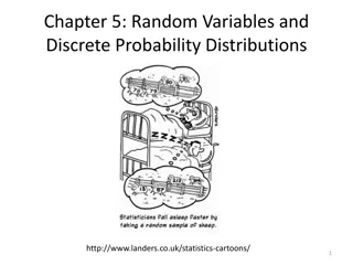
Random Variables and Mean in Statistics
Random variables can be discrete or continuous, with outcomes represented as isolated points or intervals. The Law of Large Numbers shows how the mean of observed values approaches the population mean as the number of trials increases. Calculating the mean of a random variable involves finding the expected outcome over time. Linear combinations and rules for averages and standard deviations of random variables are vital in statistical analysis.

Download Presentation

Please find below an Image/Link to download the presentation.
The content on the website is provided AS IS for your information and personal use only. It may not be sold, licensed, or shared on other websites without obtaining consent from the author.If you encounter any issues during the download, it is possible that the publisher has removed the file from their server.
You are allowed to download the files provided on this website for personal or commercial use, subject to the condition that they are used lawfully. All files are the property of their respective owners.
The content on the website is provided AS IS for your information and personal use only. It may not be sold, licensed, or shared on other websites without obtaining consent from the author.
E N D
Presentation Transcript
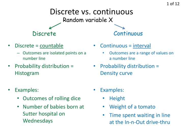
1 of 12 Discrete vs. continuous Random variable X Continuous Discrete Discrete = countable Outcomes are isolated points on a number line Probability distribution = Histogram Continuous = interval Outcomes are a range of values on a number line Probability distribution = Density curve Examples: Outcomes of rolling dice Number of babies born at Sutter hospital on Wednesdays Examples: Height Weight of a tomato Time spent waiting in line at the In-n-Out drive-thru
2 of 12 Law of Large Numbers As the number of trials (samples, observations ) increases, mean x of the observed values approaches population mean . How large is a large number? Depends on variability of observations. More variability need more observations Example: Thumbtacks
3 of 12 Mean of a Random Variable Other names: expected value, weighted average Contextual definition: Expected outcome, per trial, over a long period of time. Procedure Sum of the products of probability and value, for each event in the sample space. Example: You pay $1 to play. Flip 3 coins. If all 3 are the same, you get $3. Event 0 Heads 1 Head 2 Heads 3 Heads Value ($) 2 -1 -1 2 P(X) 1/8 2 3/8 3 3/8 3 1/8 2 . 0 25 + + + = 8 8 8 8
4 of 12 Another example Pay $1 to play my game, roll two standard dice. If their sum is 7 or 8, double your money! (get $2) Let random variable X be the money ($) you win. Event Win: 1 Lose: -1 Value 1 -1 25 11 P(X) 36 36 . 0 389 25 11 = + 36 36
5 of 12 Example #1 You work for a company that manufactures refrigerators, and you are examining surface flaws , such as dimples and paint chips. You find that your company s refrigerators have a mean 0.7 dimples, with =0.11, and a mean 1.4 paint chips, with =0.2. The distributions of both dimples and paint chips are Normally distributed. 1. What is the average number of imperfections on a refrigerator? 2. What is the standard deviation of your answer to #1? 3. What is the probability that a randomly selected refrigerator has less than 2 surface flaws?
6 of 12 Linear Combinations: 3 Rules 1. The average of both random variables is the sum of each of their averages. Works whether or not X and Y are independent. x+y = x + y x-y = x - y 2. The standard deviation of both random variables is the square root of the sum of their variances. Only works if X and Y are independent. x+y= x2+ y2 x-y= x2+ y2 3. Any linear combination of normally distributed random variables is also normally distributed.
7 of 12 Example #1 ANSWERS You work for a company that manufactures refrigerators, and you are examining surface flaws , such as dimples and paint chips. You find that your company s refrigerators have a mean 0.7 dimples, with =0.11, and a mean 1.4 paint chips, with =0.2. The distributions of both dimples and paint chips are Normally distributed. 1. What is the average number of imperfections on a refrigerator? 1 . 2 4 . 1 7 . 0 = + 2. What is the standard deviation of your answer? 2 . 0 + = 2 2 . 0 11 . 0 228 1 . 2 2 = . 0 44 3. refrigerator has less than 2 surface flaws? What is the probability that a . 0 228 . 0 33
8 of 12 Example #2 Mr. Starnes likes sugar in his hot tea. From experience, he needs between 8.5 and 9 grams of sugar in a cup of tea for the drink to taste right. While making his tea one morning, Mr. Starnes adds four randomly selected packets of sugar. Suppose the amount of sugar in these packets follows a Normal distribution with mean 2.17 grams and standard deviation 0.08 grams. What is the probability that Mr. Starnes cup of tea will taste right? + + + = . 2 17 . 2 17 . 2 . 0 17 08 . 2 17 . 0 + 9 68 . 0 + 68 . 8 . 8 MEAN: STANDARD DEVIATION: . 8 5 . 8 + = 2 2 2 2 08 08 . 0 08 . 0 16 68 = . 1 125 = 2 . 0 16 . 0 848 16 1292 . 0 = 9772 . 0 . 0
9 of 12 Binomial Properties of a binomial experiment: 1. Fixed number (n) of trials. 2. Only 2 outcomes for each trial. 3. Trials are independent. 4. Probability (p) is constant. Independent Population 10+ times bigger than sample. N>10n Is it binomial? A. The number X of children out of 5 children who inherit a particular blood type from their parents. B. Deal 10 cards from a shuffled deck and count the number X of red cards. C. An engineer chooses an SRS of 10 switches from a shipment of 10,000 switches, where 10% of the total population of switches are bad. The engineer counts the number X of bad switches in the sample.
! n k n k 1 ( ) Binomial Formula: p p ( ! )! k n k k is number of successesin n trials, with probability of success p. Calculator instructions: 2nd, Distr binompdf (n,p,k) OR binomcdf (n,p,k) Exactly k successes in n trials At most k successes in n trials Examples: Roll 7 dice, get exactly three 3 s. Roll 7 dice, get at most three 3 s. Roll 7 dice, get at least three 3 s. binompdf (7, (1/6), 3) = 0.078 binomcdf (7, (1/6), 3) = 0.982 binomcdf (7, (1/6), 2) = 0.904 1 0.904 = 0.095
11 of 12 Binomial Formula ! n k number of successes n trials p probability of success k n k 1 ( ) p p ( ! )! k n k Examples: Roll 7 dice, get exactly three 3 s. ! 7 1 1 3 7 3 ( ) 1 ( ) 7 ( ! 3 3 )! 6 6 Roll 7 dice, get at most three 3 s. 1 1 ( ) 6 )! 3 ! 7 1 ! 7 1 1 ! 7 1 1 + + 1 7 1 3 7 3 2 7 2 ( ) 1 ( ) ( ) ( ) 1 ( ) 7 ( ! 1 1 )! 6 1 ( 6 7 ( ! 3 6 7 ( ! 2 2 )! 6 6 ! 7 1 + 0 7 0 ) 1 ( ) 7 ( ! 0 0 )! 6 6 Roll 7 dice, get at least three 3 s. 1 ( )
12 of 12 Mean and s.d. of Binomial If you roll a die 900 times, how many three s do you expect? How much variability? = np 1 ( ) p = np