Functions of Random Variables and Sampling Distributions
This chapter delves into the functions of random variables and sampling distributions. It covers important statistics like populations, samples, and measures of central tendency such as the mean and median. Properties of these measures are discussed, along with examples illustrating their calculation. The median and mean are key tools for analyzing data sets and understanding their underlying characteristics.

Download Presentation

Please find below an Image/Link to download the presentation.
The content on the website is provided AS IS for your information and personal use only. It may not be sold, licensed, or shared on other websites without obtaining consent from the author.If you encounter any issues during the download, it is possible that the publisher has removed the file from their server.
You are allowed to download the files provided on this website for personal or commercial use, subject to the condition that they are used lawfully. All files are the property of their respective owners.
The content on the website is provided AS IS for your information and personal use only. It may not be sold, licensed, or shared on other websites without obtaining consent from the author.
E N D
Presentation Transcript
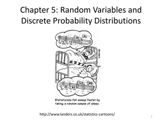
CHAPTER SIX FUNCTIONS OF RANDOM VARIABLES SAMPLING DISTRIBUTIONS
6.1 Some Important Statistics: 6.1.1 A Population: A population consists of the total observations with which we are concerned at a particular time. 6.1.2 A Sample: A sample is a subset of a population. 6.2 Definition: Central Tendency in the Sample: Any function of the random sample is called a statistic.
6.2.1 The Mean: 6.2.1 Definition: The Mean: If represent a random sample of size n, then the sample mean is defined by the statistic: X ... 1 X n n = X i = (1) X 1 i n
Properties of the Mean: 1. The mean is the most commonly used measure of certain location in statistics. 2. It employs all available information. 3. The mean is affected by extreme values. 4. It is easy to calculate and to understand. 5. It has a unique value given a set of data.
EX(1): The length of time, in minutes, that 10 patients waited in a doctor's office before receiving treatment were recorded as follows: 5, 11, 9, 5, 10, 15, 6, 10, 5 and 10. Find the mean. Solution: = 5 11 ... 10 = + + + = 10, 86 n x i x 86 10 = = = i 8.6 X n
6.2.2 The Median: X ... 1 X If represent a random sample of size n , arranged in increasing order of magnitude, then the sample median, which is denoted by is defined by the statistic: n Q 2 X if n is odd + ( 1) n 2 = (2) Q 2 X X + 2) 1 + 2 ( n n if n is even 2
Properties of the Median: 1. The median is easy to compute if the number of observations is relatively small. 2. It is not affected by extreme values.
EX(2): The number of foreign ships arriving at an east cost port on 7 randomly selected days were 8, 3, 9, 5, 6, 8 and 5. Find the sample median. Solution: The arranged values are: 3 5 5 6 8 8 9 7 , n = + + 1 7 1 2 n = = 4 2 = 6 Q 2
EX(3): The nicotine contents for a random sample of 6 cigarettes of a certain brand are found to be 2.3, 2.7, 2.5, 2.9, 3.1 and 1.9 milligrams. Find the median. Solution: The arranged values are: 1.9 ,2.3 ,2.5 ,2.7, 2.9, 3.1 . 6 6 , 3 , 2 2 2.5 2.7 2.6 2 6 2 n n = = = + = + = + = 1 1 3 1 4 n 2 + = = Q 2
6.2.3 The Mode: If not necessarily all different, represent a random sample of size n, then the mode M is that value of the sample that occurs most often or with the greater frequency. The mode may not exist, and when it does it is not necessarily unique. X ... 1 X n
Properties of the Mode: 1. The value of the mode for small sets of data is almost useless. 2. It requires no calculation.
EX(4): The numbers of incorrect answers on a true false test for a random sample of 14 students were recorded as follows: 2, 1, 3, 0, 1, 3, 6, 0, 3, 3, 2, 1, 4, and 2, find the mode. Solution: 3 M =
Notes: 1. The sample means usually will not vary as much from sample to sample as will the median. 2. The median (when the data is ordered) and the mode can be used for qualitative as well as quantitative data.
3. Variability in the sample: 6.3.1 The Range: The range of a random sample is defined by the statistic , where respectively the largest and the smallest observations X ... 1 X n X X ( ) n (1) X and X ( ) (1) n which is denoted by R,then: = = R Max Min x x ( ) n (1)
EX(5): Let a random sample of five members of a sorority are 108,112,127,118 and 113. Find the range. Solution: R=127-108=19
6.3.2 The Variance: X ... 1 X If represent a random sample of size n, n 2 then the sample variance, which is denoted by is defined by the statistic: S 2 n n X 2 ( ) X X i i n 1 = = = 2 2 i 1 i = [ ] S X 1 i 1 1 n n n = 1 i n 1 = 2 i 2 [ ] X nX 1 n = 1 i
EX(6): A comparison of coffee prices at 4 randomly selected grocery stores in San Diego showed increases from the previous month of 12, 15, 17, 20, cents for a 200 gram jar. Find the variance of this random sample of price increases. Solution: 1 12 15 17 4 n n X + + + i 20 = = = = 16 X i n 2 ( ) X X (12 16) + (15 16) + (17 16) + (20 16) 2 2 2 2 i = = 2 = S 1 i 1 3 n 34 3 =
6.3.3 The Standard Deviation: The sample standard deviation, denoted by S, is the positive square root of the sample variance which is given by: = 2 S S
EX(7): The grade point average of 20 college seniors selected at random from a graduating class are as follows: 3.2, 1.9, 2.7, 2.4, 2.8, 2.9, 3.8, 3.0, 2.5, 3.3, 1.8, 2.5, 3.7, 2.8, 2.0, 3.2, 2.3, 2.1, 2.5, 1.9. Calculate the variance and the standard deviation. Solution: 53.3, i i i = = n n = = 2 i 148.55 X X 1 1 (answer: ) 2.665, X = = = 2 0.585, 0.342 S S
6.4 Sampling Distributions: 6.4.1 Definition: The probability distribution of a statistic is called a sampling distribution. 6.4.1.1 Sampling Distributions of Means: 2 = = = = 2 X ( ) , ( ) (3) E X V X X n
6.4.2 Definition: 6.4.2.1 Central Limit Theorem: If is the mean of a random sample of size n taken from a population with mean and finite variance , then the limiting form of the distribution of: X X = (4) Z as n / n is approximately the standard normal distribution; 2 = = = ( ) ~ f Z (0,1) ( ) , ( ) , N E X V X X n n ( , ~ ) (5) X N n
EX(8): An electrical firm manufactures light bulbs that have a length of life that is approximately normally distributed with mean equal to 800 hours and a standard deviation of 40 hours. Find the probability that a random sample of 16 bulbs will have an average life of less than 775 hours.
Solution: X Let X be the length of life and is the average life; = = = 16, 800, 40 n 775 800 40/ 16 = = = ( 775) ( ( 2.5) 0.0062 P X P Z P Z
EX(9): Given the discrete uniform population: 1 = , 3 , 2 , 1 , 0 X = ( ) f X 4 0 otherwise Find the probability that a random sample of size 36 selected with replacement will yield a sample mean greater than 1.4 but less than 1.8.
Solution: X 0 1 2 + + + 3 = = = i 1.5 4 K 2 ( ) X (0 1.5) + (1 1.5) + (2 1.5) + (3 1.5) 2 2 2 2 = = = 2 1.25, 4 K ( , ) (1.5,.186) , X N X N n 1.4 1.5 0.186 ( 0.54 1.7 1.5 0.186 1.08) = (1.4 1.8) ( ) P X P Z = = = 0.8599 0.2946 0.5653 P Z
Theorem: If independent samples of size n1 and n2 are drawn at random from populations, discrete or continuous with means and variances respectively, then the sampling distribution of the difference of means is approximately normally distributed with mean and variance given by: and 2 1 2 2 and 1 2 X X 1 2 2 1 2 2 = = = + 2 ( ( ) , (6) E X X 1 2 1 2 ( ) ) X X X X n n 1 2 1 2 1 2 Hence ( ) ( ) X X = (7) Z 1 2 1 2 2 2 2 1 + n n 1 2 is approximately a standard normal variable.
EX(10): 1= 50 A sample of size n1=5 is drawn at random from a population that is normally distributed with mean and variance and the sample mean is recorded. A second random sample of size n2=4 is selected independent of the first sample from a different population that is also normally distributed with mean and variance and the sample mean is recorded. Find ) 2 . 8 ( 2 1 X X P 2 1= 9 X 1 2= 2 2= 40 4 X 2
Solution: 5 n = = 4 n 1 2 = = 50 40 1 2 = = 2 1 2 2 9 4 = = = 50 40 10 1 2 X X 1 2 2 1 2 2 9 5 4 4 = + = + = 2 X 2.8 X n n 1 2 1 2 8.2 10 1.673 = = = ( 8.2) ( ) ( 1.08) 0.1401 P X X P Z P Z 1 2
EX(11): The television picture tubes of manufacturer A have a mean lifetime of 6.5 years and a standard deviation of 0.9 year, while those of manufacturer B have a mean lifetime of 6 years and a standard deviation of 0.8 year. What is the probability that a random sample of 36 tubes from manufacture A will have a mean lifetime that at least 1 year more than the mean lifetime of a sample of 49 from tubes manufacturer B?
Solution: Population 1 Population 2 = = 6.5 6.0 1 2 = = 0.9 0.8 1 2 n = n = 36 49 1 2 = = 6.5 6 0.5 X X 1 2 0.81 36 0.64 49 = + = 0.189 X X 1 2 1 0.5 0.189 2.65) = = [( ) 1) ( ) ( 2.65) P X X P Z P Z 1 2 = 1 0.996 = = 1 ( 0.004 P Z
Sampling Distribution of the sample Proportion: Let X= no. of elements of type A in the sample P= population proportion = no. of elements of type A in the population / N = sample proportion = no. of elements of type A in the sample / n = x/n p
= = ~ ( , ) ( ) , ( ) np V x x binomial n p E x npq x 1. ( ) E p = = ( ) n E p x pq n = = = 2. ( ) ( ) n , 1 V p V q p 3. For large n, we have: pq n ~ p ( , ) N p p p = ~ (0,1) Z N pq n
6.5 t Distribution: Theorem: * t distribution has the following properties: 1. It has mean of zero. 2. It is symmetric about the mean. 3. It ranges from . 4. Compared to the normal distribution, the t distribution is less peaked in the center and has higher tails. 5. It depends on the degrees of freedom (n-1). 6. The t distribution approaches the normal distribution as (n-1) approaches . to
EX(12): Find: ( ) a t = 14 when v 0.025 = ( ) b t 10 when v 0.01 = ( ) c t 7 when v 0.995
(a)t0.025 at ? = 14 ? = 2.1448 = = ( ) b t 10 2.764 at v t 0.01 = = ( ) c t 7 3.4995 at v t 0.995
EX(13): Find: ( ) ( a P T = 2.365) 7 when v = ( ) ( b P T 1.318) 24 when v ( ) ( 1.356 c P = 2.179) 12 T when v = ( ) ( d P T 2.567) 17 when v
solution = = ( ) ( a P T 2.365) 0.975 7 at v = 1.318) 1 0.9 0.1 = = = ( ) ( b P T 1.318) 1 ( 24 P T at v ( ) ( 1.356 c P = 2.179) ( 2.179) ( 1.356) T P T P T = 0.975 0.1 0.875 = = 12 at v 2.567) 1 = 2.567) 0.99 = = ( ) ( d P T ( 17 P T at v
EX (14): Given a random sample of size 24 from a normal distribution, find k such that: ( ) ( 1.7139 a P = ) 0.90 T k = ( ) ( b P k 2.807) 0.95 T = ( ) ( c P ) 0.90 k T k
Solution: ( ) ( 2.069 a P = 1.7139) ) ( ) ( T k P T k P T = = ( ) 0.05 0.9 P T k = + = ( ) 0.9 0.05 0.95 P T k = = 1.7139 23 k at v = = = ( ) ( b P k 2.807) 0.95 23 T k at v = = = ( ) ( c P ) 0.9 1.319 23 k T k k at v


:")


:")
:")


:")


:")

:")

:")


:")

:")


:")

:")


:")
t0.025 at ? = 14→ ? = −2.1448")
:")

:")