Prediction of Metallicity and C/O Ratios for Hot Jupiter Exoplanets

Slide Note

Dr. Graeme Melville from the University of NSW explores the modeling of atmospheres for hot Jupiter exoplanets, emphasizing the importance of temperature, PT profiles, metallicity, and the C/O ratio. Utilizing the Versatile Software for Transfer of Atmospheric Radiation (VSTAR), the research aims to predict spectra, offering insights into the complexities of exoplanetary atmospheres. By building atmospheric models through iterative processes, the study delves into theoretical vs. observational results, highlighting the diversity and challenges in understanding exoplanetary compositions.

deim_9 Follow

Uploaded on Oct 08, 2024 | 0 Views

Download Presentation

Please find below an Image/Link to download the presentation.

The content on the website is provided AS IS for your information and personal use only. It may not be sold, licensed, or shared on other websites without obtaining consent from the author. Download presentation by click this link. If you encounter any issues during the download, it is possible that the publisher has removed the file from their server.

E N D

Presentation Transcript

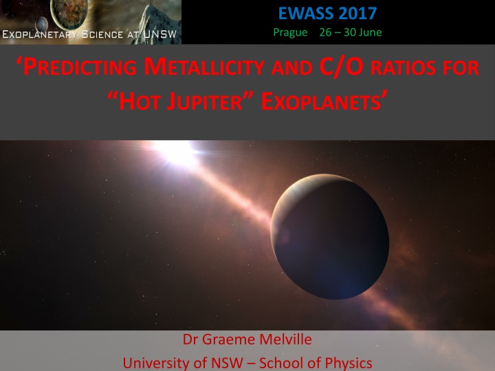
EWASS 2017 Prague 26 30 June PREDICTING METALLICITYAND C/O RATIOSFOR HOT JUPITER EXOPLANETS Dr Graeme Melville University of NSW School of Physics

PREVIEW o VSTAR Modelling stars, brown dwarfs, Solar planets, exoplanets ( Hot Jupiters ) o Atmospheres of Hot Jupiters o Importance of temperature, PT profiles, metallicity and the C/O ratio o Results - Theoretical Vs Observational o Where are we going? Slide 2 of 28

EXOPLANET HR DIAGRAM? But exoplanets are far more complicated!! Large range: Irradiation temperature, Gravity Chemical composition Large diversity of exoplanet atmospheres Need fast, accurate, and versatile atmospheric models.

MODELLING? o Versatile Software for Transfer of Atmospheric Radiation (VSTAR) - theoretical atmospheric profiles of exoplanets. o Predicts the spectra of Solar System planets, exoplanets, brown dwarfs and cool stars. - line-by-line approach to molecular & atomic absorption with a full multiple scattering treatment of radiative transfer. - incorporates an ionisation and chemical equilibrium model. - comprehensive treatment of spectral line absorption using a database of more than 2.9 billion spectral lines. - good for: 60 K (Uranus) T 6000 K (stars) o 0.324 m 28.6 m with 304,501 spectral data points.

HOWTOBUILDAN ATMOSPHERICMODEL 1. Start estimate PT structure of the atmosphere over a number of layers (~40 80). 2. For each layer calculate the composition & concentration for important atoms and molecules assuming chemical equilibrium. 3. Calculate the opacity (extinction coeff) of each layer at each wavelength taking account of atomic and molecular absorption lines and continuum opacity sources such as bound-free and free-free absorption, collision induced absorptions, Rayleigh and electron scattering at which significant energy transport occurs. Absorption loses energy; emission gains energy; scattering redistributes energy 4. Solve the radiative transfer equation to determine the radiative energy flux through each layer. 5. Iteratively adjust the temperature structure of the model, repeating steps 2-4 as required until the model is in energy balance. Total flux through each layer must equal T4eff.

THEORY - PLANETARY ATMOSPHERES o Secondary Eclipse emission spectrum (Sensitive to absolute chemical abundances & thermal profile) o C/O > 1 CO; CH4; C2H2; HCN (little H20) (carbide dominated) o C/O < 1 lots of CO2; H2O (silicate dominated such as Mg-Si-O & Fe-Ni metals) < 2000 K: solid/liquid condensates start to form o However, not everything is stable: H20: 2200 K ~ 3% H2O has decomposed and 3000 K ~ 50% has decomposed CH4: drops off quickly > 1000 K NH3: drops off > 500 K but CO2 and CO increases HCN (> 750 K) and C2H2 (> 1000 K) visible and UV absorption T. inversion H2O vibrational modes Slide 6 of 28

EXPECTATIONS o Molecules, Clouds, and Hazes in Atmospheres o The Knowns for Giant Planets: Molecules we re guaranteed to see NH3; CH4; H2O; CO; CO2 (at least at 10mbar and 1500 K) We d like to know the abundances of these molecules within a factor of ~5 Would allow connection to planet formation o The Known Unknowns: Molecules we expect to see depending on the effects of photochemistry and C/O ratio: HCN; C2H2; C2H4; C2H6 o The Unknown Unknowns: Our imperfect understanding of these atmospheres, in the absence of spectral data Phosphorus compounds? Sulphur compounds? For smaller planets, the number of unknowns goes up, due to uncertain initial conditions and surface/interior/atmosphere interactions. Slide 7 of 28

SIMULATIONS Hot Jupiters have clouds, haze, dust, aerosols/smog. Model Parameters: a Jupiter-sized planet around a Sun-like star(g = 24.8) no: dust, clouds, smog etc. 4 different exoplanet temperatures Low (LT) (896 K 1500 K) (0.12 au) Standard (ST) (1160 K 2250 K) (0.07 au) High (HT) (1508 K 2600 K) (0.04 au) V High (VHT) (1836 K 3000 K) (0.027 au)

SIMULATIONS Model parameters: - Metallicity (Sun ~0) Actual Z Program Z -0.6 0.25 4 times less -0.4 0.4 2.5 times less 0 1 same 0.48 3 3 times more 0.6 4 4 times more - C/O ratio (Sun ~0.54) e.g. HTZ3C0.6 C/O ratio 1/5 of solar 0.1 bit less than solar 0.4 0.7 ~3 times solar 1.6 ~4 times solar 2.0

SIMULATIONS Pressure/Temperature profile: no significant temperature inversion - based on HD189733b (1160 K 2250 K) and (0.0001 mb 4.93 bars) 1 10-8 1 10-7 1 10-6 1 10-5 P ress (b ar) 1 10-4 1 10-3 1 10-2 1 10-1 1 100 1 101 1000 1200 1400 1600 1800 2000 2200 2400 T em pt K

RESULTS - SPECTRA o Secondary Eclipse emission spectrum Sim A _H TZ1C 0.4_binned 0.0040 0.0035 0.0030 0.0025 (F p /F s ) Flux 0.0020 0.0015 0.0010 0.0005 0.0000 0.5 1 1.5 2 2.5 3 4 5 6 6 7 7 8 8 9 9 10 13 15 20 30 W avelength (28.6 - 0.324 ) Can estimate the temperature of the Hot Jupiter by fitting observed spectra to those predicted by model atmospheres. Slide 11 of 28

RESULTS - SPECTRA o Secondary Eclipse emission spectrum (increasing Z, constant C/O) S im B _V H TZ0.25C 0.4_binned 0.0040 S im B _V H TZ1C 0.4_binned 0.0040 0.0035 0.0035 H 2O H 2O 0.0030 0.0030 H 2O 0.0025 0.0025 (F p /F s) (F p /F s) F lu x F lu x 0.0020 0.0020 H 2O 0.0015 0.0015 0.0010 0.0010 0.0005 0.0005 0.0000 0.0000 0.5 1.5 2 2.5 3 3 4 4 5 6 7 8 9 13 15 20 30 1 10 0.5 1.5 2 2.5 3 3 4 4 5 6 7 8 9 15 20 30 1 10 W avelen g th (28.6 - 0.324 ) W avelen g th (28.6 - 0.324 ) S im B _V H TZ4C 0.4_binned 0.0040 0.0035 0.0030 H 2O 0.0025 H 2O (F p /F s) F lu x 0.0020 0.0015 0.0010 0.0005 Slide 12 of 28 0.0000 0.5 1.5 2 2.5 3 4 5 6 7 8 9 13 15 20 30 1 10 W avelen g th (28.6 - 0.324 )

RESULTS - SPECTRA (Increasing C/O; constant Z) S im C _V H TZ1C 0.4_binned S im C _V H TZ1C 0.7_binned 0 .0 0 4 0 0 .0 0 4 0 0 .0 0 3 5 0 .0 0 3 5 T iO H C N ? H 2O 0 .0 0 3 0 0 .0 0 3 0 H 2O C O H 2O H 2C 2 H C N H 2O H C N 0 .0 0 2 5 0 .0 0 2 5 C O H C N H 2C 2 H C N H 2O H 2O (Fp/Fs) (Fp/Fs) F lu x F lu x 0 .0 0 2 0 0 .0 0 2 0 T iO H C N ? 0 .0 0 1 5 0 .0 0 1 5 0 .0 0 1 0 0 .0 0 1 0 0 .0 0 0 5 0 .0 0 0 5 0 .0 0 0 0 0 .0 0 0 0 0.5 1.5 2 2.5 3 4 5 6 7 8 9 13 15 20 30 1 1 0 0.5 1.5 2 2.5 3 4 5 6 7 8 9 13 15 20 30 1 1 0 W av elen g th (2 8 .6 - 0 .3 24 ) W av elen g th (2 8 .6 - 0 .3 24 ) S im D _V H TZ1.05C 0.98_binned S im D _V H TZ1.04C 1.1_binned 0 .0 0 5 0 0 .0 0 4 0 HCN 0 .0 0 4 5 0 .0 0 3 5 0 .0 0 4 0 H 2O 0 .0 0 3 0 C O 0 .0 0 3 5 H 2C 2 ? HCN H C N 0 .0 0 2 5 0 .0 0 3 0 H 2O H 2O H 2O H 2O H 2C 2 H C N (Fp/Fs) (Fp/Fs) F lu x F lu x 0 .0 0 2 5 0 .0 0 2 0 0 .0 0 2 0 C O 0 .0 0 1 5 T iO T iO H C N ? 0 .0 0 1 5 V O ? 0 .0 0 1 0 0 .0 0 1 0 0 .0 0 0 5 0 .0 0 0 5 Slide 13 of 28 20 30 0 .0 0 0 0 0 .0 0 0 0 0.5 1.5 2 2.5 3 4 5 6 7 8 9 13 15 1 1 0 0.5 1.5 2 2.5 3 4 5 6 7 8 9 13 15 20 30 1 1 0 W av elen g th (2 8 .6 - 0 .3 24 ) W av elen g th (2 8 .6 - 0 .3 24 )

RESULTSCC DIAGRAMS o IR Colour-Colour Diagrams Used [J], [H], [Ks], [3.6] and [4.5]. Best to use J, H and Ks have limited absorption features hence probe the deep layers of the atmosphere. Hard to get data on [J] and [H], [Ks] is a bit better, more on [3.6] and [4.5]. o Constant Z, varying C/O J - H 2 .0 S T (1160K - 2250 K ) 1 .9 1 .8 1 .7 (Z4) S T Z4 C 0 .1 g 8 1 .6 1 .5 1 .4 1 .3 1 .2 S T Z4 C 0 .1 1 .1 1 .0 Z4 C 0 .5 0 .9 Z4 C 0 .7 0 .8 0 .7 0 .6 0 .5 Z4 C 0 .9 5 Z4 C 1 .0 0 .4 0 .3 0 .2 0 .1 0 .0 -0 .1 Z4 C 1 .3 -0 .2 -0 .3 -0 .4 -0 .5 Z4 C 2 .0 -0 .6 -0 .7 -0 .8 -0 .9 -1 .0 0 .0 0 .1 0 .2 0 .3 0 .4 0 .5 0 .6 0 .7 0 .8 0 .9 1 .0 1 .1 1 .2 1 .3 1 .4 H - K s 1 .5 Slide 14 of 28

RESULTS - o Standard temperature and varying Z and C/O. J - H 1 .2 S T Z4C 0.1 S T Increasing C/O 1 .1 1 .0 S T Z2.2C 0.1 Z4C 0.5 0 .9 Z2.2C 0.4 Z4C 0.7 0 .8 Z1C 0.1 Z2.2C 0.7 0 .7 Z1C 0.4 0 .6 Z1C 0.7 Increasing Z Z0.4C 0.1 Z2.2C 0.88 Z0.4C 0.4 0 .5 S T Z0.25C 0.1 Z0.4C0.8 Z0.25C 0.4 Z0.4C 0.95 Z0.25C 0.6 Z2.2C 1.0 Z1C 1.0 0 .4 Z4C 0.95 Z0.4C 1.0 Z0.25C 0.84 Z0.25C 1.0 Z0.25C 1.1 Z0.4C 1.2 Z4C 1.0 0 .3 Z2.2C 1.1 Z0.25C 1.3 Z1C 1.2 0 .2 Z0.25C 1.6 Z0.4C 1.6 0 .1 Z0.25C 2.0 0 .0 Z0.4C 2.0 Increasing C/O Z1C 1.6 -0 .1 Z4C 1.3 -0 .2 Z2.2C 1.6 Z1C 2.0 -0 .3 -0 .4 Z2.2C 2.0 -0 .5 Increasing Z -0 .6 Z4C 2.0 -0 .4 -0 .3 -0 .2 -0 .1 0 .0 0 .1 0 .2 0 .3 0 .4 0 .5 0 .6 0 .7 0 .8 0 .9 H - K s 1 .0 Slide 15 of 28

RESULTS o Theoretical. J - H 1 .2 S T Z4C 0.1 High Z Medium C/O S T 1 .1 1 .0 S T Z2.2C 0.1 Z4C 0.5 0 .9 Z2.2C 0.4 High Z Low C/O Z4C 0.7 0 .8 Z1C 0.1 Z2.2C 0.7 0 .7 Z1C 0.4 0 .6 Z1C 0.7 Z0.4C 0.1 Z2.2C 0.88 Z0.4C 0.4 0 .5 S T Z0.25C 0.1 Z0.4C0.8 Low Z Low C/O Z0.25C 0.4 Z0.4C 0.95 Z0.25C 0.6 Z2.2C 1.0 Z1C 1.0 0 .4 Z4C 0.95 Z0.4C 1.0 Z0.25C 0.84 Z0.25C 1.0 Z0.25C 1.1 Z0.4C 1.2 Z4C 1.0 0 .3 Z2.2C 1.1 Z0.25C 1.3 Z1C 1.2 0 .2 Z0.25C 1.6 Z0.4C 1.6 High Z High C/O 0 .1 Z0.25C 2.0 0 .0 Z0.4C 2.0 Z1C 1.6 -0 .1 Low/Med Z High C/O Z4C 1.3 -0 .2 Z2.2C 1.6 Z1C 2.0 -0 .3 -0 .4 Z2.2C 2.0 -0 .5 -0 .6 Z4C 2.0 -0 .4 -0 .3 -0 .2 -0 .1 0 .0 0 .1 0 .2 0 .3 0 .4 0 .5 0 .6 0 .7 0 .8 0 .9 H - K s 1 .0 Slide 16 of 28

RESULTS o Theoretical. K s - [4.5] 2 .1 5 S T Z4C 2.0 S T Z4C 0.1g 8 High Z High C/O 2 .1 0 Z2.2C 2.0 2 .0 5 Z4C 1.3 Z2.2C 1.6 2 .0 0 Z1C 2.0 S T Z4C 0.1 High Z Low C/O 1 .9 5 Z1C 1.6 S T Z2.2C 0.1 High Z Med C/O Z4C 1.0 Low Z High C/O Z0.4C 2.0 Z4C 0.95 Z2.2C1.1 1 .9 0 Z4C 0.5 Low Z Low C/O Z0.25C 2.0 Z1C 0.1 Z0.25C 1.6 Z1C 1.2 Z2.2C 1.0 Z2.2C 0.4 S T Z0.25C 0.1 Z0.4C1.6 Z0.25C 1.0 Z0.4C 0.1 Z0.25C1.1 Z0.25C 0.84 Z0.25C 0.4 Z0.4C1.0 Z0.4C 1.2 Low Z Med C/O Z0.25C 0.6 1 .8 5 Z1C 1.0 Z2.2C 0.88 Z4C 0.7 Z1C 0.4 Z0.4C 0.4 Z1C 0.7 Z2.2C 0.7 1 .1 0 1 .1 5 1 .2 0 1 .2 5 1 .3 0 1 .3 5 1 .4 0 1 .4 5 1 .5 0 1 .5 5 1 .6 0 K s - [3.6] 1 .6 5 Slide 17 of 28

RESULTS o All temperatures theoretical and experimental K s - [4.5] 2 .2 Z4C 2.0 S TZ4C 0.1g8 Z2.2C 2.0 Z2.2C 1.6 2 .0 S TZ4C 0.1 Z0.4C 2.0 Increasing temperature S T Z0.25C 1.1 Z0.4C 0.1 1 .8 Z2.2C 0.7 1 .6 1 .4 H T Z 1C 0.4 1 .2 V H T Z 1C 0.4 W A S P 18b (2188K ) 1 .0 V H TZ1.011C 0.9 W A S P 43b (1318K ? ) 0 .8 V H TZ0.4C 0.98 W A S P 19b (2071K ) V H TZ1.04C 1.1 0 .6 0 .4 W A S P 12b (> 2500K ) 0 .2 0 .0 Slide 18 of 28 K s - [3.6] 0 .0 0 .1 0 .2 0 .3 0 .4 0 .5 0 .6 0 .7 0 .8 0 .9 1 .0 1 .1 1 .2 1 .3 1 .4 1 .5 1 .6 1 .7 1 .8

RESULTS Theoretical and experimental K s - [4.5] K s - [4.5] 1 .5 5 1 .5 5 High Z Low C/O H T H T Z4C 0.1 Z4C 0.1 1 .5 0 1 .5 0 Z4C 0.2 Z4C 0.2 Z2.2C 0.1 Z2.2C 0.1 Z4C 0.4 Z4C 0.4 High/Med Z Med C/O 1 .4 5 1 .4 5 1508K 2600K) Z2.2C 0.4 Z2.2C 0.4 Z1C 0.1 Z1C 0.1 Z2.2C 0.5 Z2.2C 0.5 1 .4 0 1 .4 0 Z4C 0.7 Z4C 0.7 Z1C 0.4 Z1C 0.4 Z0.4C0.1 Z0.4C0.1 1 .3 5 1 .3 5 Z2.2C 0.7 Z2.2C 0.7 Z0.25C0.1 Z0.25C0.1 Z2.2C 0.76 Z2.2C 0.76 Low Z Med C/O 1 .3 0 1 .3 0 Z0.4C 0.4 Z0.4C 0.4 Z1C 0.7 Z1C 0.7 Z0.25C 0.4 Z0.25C 0.4 Low Z High C/O Z1C 0.77 Z1C 0.77 1 .2 5 1 .2 5 Z0.4C 0.7 Z0.4C 0.7 Z0.25C 0.7 Z0.25C 0.7 Z4C 0.9 Z4C 0.9 Z0.25C 0.8 Z0.25C 0.8 Z0.4C0.8 Z0.4C0.8 1 .2 0 1 .2 0 Z2.2C 0.9 Z2.2C 0.9 Z0.25C 0.84 Z0.25C 0.84 Z0.23C 0.9 Z0.23C 0.9 Z1C 0.9 Z1C 0.9 Z0.4C 0.9 Z0.4C 0.9 Z0.25C0.97 Z0.25C0.97 Z0.25C 1.0 Z0.25C 1.0 Z0.4C 0.95 Z0.4C 0.95 Z0.25C1.3 Z0.25C1.3 Z0.25C 1.9 1 .1 5 1 .1 5 Z0.4C 1.0 Z0.4C 1.0 High/Med Z High C/O Z0.4C 1.1 Z0.4C 1.1 Z0.25C 1.9 Z0.4C 1.3 Z0.4C 1.3 Z0.25C2.0 Z0.25C2.0 Z0.4C 1.5 Z0.4C 1.5 Z1C 1.0 Z1C 1.0 1 .1 0 1 .1 0 Z0.4C 2.0 Z0.4C 2.0 Z1C 1.18 Z1C 1.18 1 .0 5 1 .0 5 Z1C 1.3 Z1C 1.3 Z2.2C 1.02 Z2.2C 1.02 Z1C 1.6 Z1C 1.6 Z2.2C 1.1 Z2.2C 1.1 Z1C 2.0 Z1C 2.0 Z4C 1.0 Z4C 1.0 1 .0 0 1 .0 0 Z2.2C 1.3 Z2.2C 1.3 W A S P 18b Z4C 1.1 Z4C 1.1 0 .9 5 0 .9 5 Z2.2C1.5 Z2.2C1.5 Z2.2C 1.9 Z2.2C 1.9 Z4C 1.3 Z4C 1.3 Z4C 1.5 Z4C 1.5 0 .9 0 0 .9 0 Z4C 1.9 Z4C 1.9 Z4C2.0 Z4C2.0 0 .8 5 0 .8 5 0 .7 0 0 .7 0 0 .7 5 0 .7 5 0 .8 0 0 .8 0 0 .8 5 0 .8 5 0 .9 0 0 .9 0 0 .9 5 0 .9 5 1 .0 0 1 .0 0 1 .0 5 1 .0 5 1 .1 0 1 .1 0 1 .1 5 1 .1 5 1 .2 0 1 .2 0 Slide 19 of 28 K s - [3.6] K s - [3.6]

RESULTS o Changing g but constant Z and C/O K s - [4.5] 1 .8 H T Z1C 0.4 1 .7 1 .6 H T Z1 C 0 .4 g 4 .8 1 .5 H T Z1 C 0 .4 g 1 2 .8 H T Z1 C 0 .4 g 1 6 .8 H T Z1 C 0 .4 g 2 0 .8 1 .4 H T Z1 C 0 .4 g 2 4 .8 1 .3 1 .2 1 .1 Slide 20 of 28 1 .2 0 K s - [3.6] 1 .0 0 1 .0 2 1 .0 4 1 .0 6 1 .0 8 1 .1 0 1 .1 2 1 .1 4 1 .1 6 1 .1 8

RESULTS XHT (2240K 3661K) Adjusting for g and the target (Wasp 19b) 1 2 .5 1000K [4.5] S T L T Z 1 C 0.4 Increasing temperature 1500K 1 2 .0 1 1 .5 S T Z 1 C 0.4 1 1 .0 2000K H T Z1C 0.4 1 0 .5 V H T Z1C 0.4 (g rad = 63/100) 1 0 .0 X H T Z0.8C 0.8g 14.8 9 .5 W asp 19b (2071K ) X H T Z0.4C 0.8g 24.8 9 .0 X H T Z0.8C 0.8g 14.8 lu m a d j fo r W A S P 19b X H T Z0.4C 0.8g 14.8 lu m a d j fo r W A S P 19b X H T Z0.4C 0.8g 24.8 lu m a d j fo r W A S P 19b 8 .5 Slide 21 of 28 9 .0 9 .5 1 0 .0 1 0 .5 1 1 .0 1 1 .5 1 2 .0 1 2 .5 1 3 .0 1 3 .5 1 4 .0 1 4 .5 1 5 .0 K s

RESULTS o Other CC diagrams 1 6 .0 Theoretical and experimental [J] 1 5 .5 Z 4C 0.1 1 5 .0 Z 2.2C 0.1 S T 1 4 .5 Z 1C 0.1 Z 4C 0.7 1 4 .0 Z 2.2C 0.7 Z 1C 0.4 Z 0.4C 0.1 Z 4C 2.0 Z 2.2C 2.0 1 3 .5 Z 0.25C 0.4 Z 1C 2.0 H T Z1C 0.4 1 3 .0 Z 0.25C 0.84 Z 0.4C 2.0 Z 0.25C 1.3 W asp 19b (2071 K ) 1 2 .5 V H T Z1C 0.4 1 2 .0 V H T Z 1.04C 1.1 V H T Z 0.4C 0.98 1 1 .5 W asp 46b (2386K ) 1 1 .0 X H T Z0.8C 0.8g 14.8 lu m a d j fo r W A S P 19b X H T Z0.4C 0.8g 14.8 lu m a d j fo r W A S P 19b 1 0 .5 X H T Z0.4C 0.8g 24.8 lu m a d j fo r W A S P 19b W asp 5b (1584K ) 1 0 .0 9 .5 W asp 18b (2188 K ) W asp 12b (2320K ) Slide 22 of 28 9 .0 8 .0 8 .5 9 .0 9 .5 1 0 .0 1 0 .5 1 1 .0 1 1 .5 1 2 .0 1 2 .5 1 3 .0 1 3 .5 1 4 .0 K s

RESULTS o Another CC diagram 1 0 .4 [3.6] V H T V H T Z4C 0.4 V H T Z3C 0.4 V H T Z1C 0.1 Z1C 0.4 Z1C 0.7 1 0 .2 V H T Z0.4C 0.4 V H T Z0.25C 0.4 W A S P 5b Z1C 0.9 1 0 .0 Z1C 2.0 Z1C 1.6 Z1C 1.3 Z1C 0.95 Z1C 1.1 9 .8 Z1C 0.98 V H T Z0.4C 0.98 X H T Z0.4C 0.8g 14.8 X H T Z0.4C 0.8g 24.8 9 .6 9 .4 9 .2 W A S P 18b W A S P -19b 9 .0 X H T Z0.4C 0.8g 14.8 a d j W A S P 19b X H T Z0.4C 0.8g 24.8 a d j W A S P 19b 8 .8 9 .4 9 .6 9 .8 1 0 .0 1 0 .2 1 0 .4 1 0 .6 1 0 .8 1 1 .0 1 1 .2 1 1 .4 1 1 .6 Slide 23 of 28 K s

SUMMARY o VSTAR is an extremely versatile, accurate radiation transfer program with unique features. o Hot Jupiters do occupy specific positions on colour-colour diagrams and there are a number of trends with C/O, metallicity and temperature being the most important parameters ignoring clouds, dust etc. o IR CC diagrams are of value although they are far from simple and can be difficult to interpret when applying to actual exoplanets. o Temperature inversions, which are common for the hottest exoplanets, give a reverse diagonal C/O ratio. Slide 24 of 28

WHATSAHEAD? o Need more experimental data in the important IR bands. New satellites/instruments (JWT) will give much more observational data with smaller error bars to test the models. o Need to incorporate atmospheric dust, clouds etc. into any model across a wide range of temperatures and atmospheric conditions. o Most info will come from a diverse set of models and tying these in with the physical and chemical processes on these planets. o Applying this work to cooler exoplanets. o Work is well advanced in using polarimetry for exoplanets (HIPPI). Theoretically, could determine many atmospheric properties of hot Jupiters with data from just two or three IR bands. Slide 25 of 28