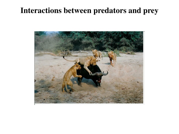
Predator-Prey Interactions: Impacts and Equilibria

Explore the dynamics of predator-prey interactions, including what defines a predator, the impacts predators have on prey populations, and the equilibrium points in the Lotka-Volterra Predator-Prey model. Discover how predation plays a crucial role in regulating population densities and observe the population cycles of Lynx and Hare as a result of predation.

• Predator-prey
• Impacts
• Equilibria
• Lotka-Volterra model
• Population cycles

jyllin Follow

Uploaded on Sep 11, 2024 | 0 Views

Download Presentation

Please find below an Image/Link to download the presentation.

The content on the website is provided AS IS for your information and personal use only. It may not be sold, licensed, or shared on other websites without obtaining consent from the author. Download presentation by click this link. If you encounter any issues during the download, it is possible that the publisher has removed the file from their server.

Presentation Transcript

1. Interactions between predators and prey

2. What is a predator? Predator An organism that consumes other organisms and inevitably kills them. Predators attack and kill many different prey individuals over their lifetimes MA0164_1m Brook Trout Salvelinus fontinalis Masked Shrew Sorex cinereus Mountain lion Puma concolor Dragonfly Diphlebia lestoides

3. How do predators impact prey populations? Direct effects Indirect effects

4. Understanding direct impacts of predation Lepus americanus (Snowshoe hare) Lynx canadensis (Lynx)

5. What role does predation play in regulating population densities?

6. Population cycles of Lynx and Hare Data from Hudson s Bay Company pelt records Are these cycles in lynx and hare densities the product of predation?

7. The Lotka-Volterra Predation Model Alfred James Lotka (1880 - 1949) Vito Volterra (1860-1940)

8. The Lotka-Volterra Predation Model ?

9. The Lotka-Volterra Predation Model Prey Predator dN dP = = rN NP NP qP dt dt is the per capita impact of the predator on the prey (-) is the per capita impact of the prey on the predator (+) q is the predator death rate (assumes a specialist predator)

10. What are the equilibria? Prey Predator = NP = rN 0 0 qP NP = = 0 ( ) N r P 0 ( ) P N q Here we see that P = 0 is one equilibrium, but there is also another: Here we see that N = 0 is one equilibrium, but there is also another: = q N = r P q r N = P = Solving for the prey equilibrium actually gives us an answer in terms of the predator! Solving for the predator equilibrium actually gives us an answer in terms of the prey!

11. Are these equilibria ever reached? (in this example, r = and q = ) Time series plots Phase plots 1.2 1.2 Population density Predator density Equilibrium Equilibrium Prey 1.1 1.1 1 1 Predator 0.9 0.9 0.8 0.8 0 200 400 600 800 1000 0.8 0.9 1 1.1 1.2 1.2 1.2 Population density Predator density Equilibrium Prey 1.1 1.1 1 1 0.9 0.9 Predator Equilibrium 0.8 0.8 0 200 400 600 800 1000 0.8 0.9 1 1.1 1.2 Time Prey density The model always produces cycles in population densities!

12. Summary of the Lotka-Volterra predation model The only possible behavior is population cycles Stable equilibria are not possible Direct impacts of predation could explain the lynx-hare cycles But not other predator-prey interactions that do not cycle Does our model make important assumptions that limit its generality?

13. Model assumptions Growth of the prey is limited only by predation (i.e., no K) The predator is a specialist that can persist only in the presence of this single prey item Individual predators can consume an infinite # of prey Predator and prey encounter one another at random (N*P terms) Predation causes additive rather than compensatory mortality Now let s modify the model to relax the blue assumptions one at a time

14. How could we add intraspecific competition? ?

15. Adding prey density dependence Prey Predator 1 dN N dP = = rN NP NP qP dt K dt Prey density dependence

16. What is the effect of incorporating prey K? 6 6 Population density Predator density K=10 5 5 4 4 Prey 3 3 2 2 1 1 Predator 0 0 0 1 2 3 4 5 6 0 200 400 600 800 1000 6 6 Population density Predator density K=10 5 5 4 4 Predator 3 3 2 2 1 1 Prey 0 0 0 1 2 3 4 5 6 0 200 400 600 800 1000 Time Prey density A stable equilibrium population size is always reached!

17. Results of adding prey density dependence 6 Predator density 5 Population cycles are no longer neutrally stable 4 3 2 Populations always evolve to a single stable equilibrium 1 0 0 1 2 3 4 5 6 This equilibrium is characterized by a prey population density well below carrying capacity 6 Predator density 5 4 3 Suggests that predators could be effective at regulating prey density 2 1 0 0 1 2 3 4 5 6 Prey density

18. Adding limits to predator consumption The original Lotka-Volterra model assumes a Type I Functional Response # of prey eaten per predator 10 is the slope of this line of this line 9 is the slope 8 7 6 5 4 3 2 1 0 0 5 10 15 20 25 30 Prey density This assumes each predator can potentially consume an infinite # of prey!

19. Wolves and Moose on Isle Royal Vucetich et al. (2002) Wolf predation rate does not increase linearly with moose population size

20. Suggests a Type II Functional Response # of prey eaten per predator 10 9 Type I 8 7 6 5 4 Type II 3 2 1 0 0 5 10 15 20 25 30 Prey density The Type II Functional Response assumes that predators get full!

21. Dynamics with non-linear functional responses 10 9 Type I # of prey eaten 8 per predator 7 6 5 4 Type II 3 2 1 0 Type I dynamics 0 5 10 15 20 25 30 Prey density 1.2 Predator density 1.1 1 0.9 0.8 0.8 0.9 1 1.1 1.2 Prey density

22. Type II Dynamics 10 10 Prey Predator per predator 8 8 Prey eaten Population density 6 6 4 4 2 2 Increasing predator saturation 0 0 0 2 4 6 8 10 0 500 1000 1500 2000 10 10 8 per predator 8 Population Prey eaten density 6 6 4 4 2 2 0 0 0 500 1000 1500 2000 0 2 4 6 8 10 10 10 8 8 per predator Population Prey eaten density 6 6 4 4 2 2 0 0 0 2 Prey density 4 6 8 10 0 500 1000 Time 1500 2000

23. Impacts of saturating functional response Decreases the predators ability to effectively control the prey population Leads to periodic outbreaks in prey population density Prey outbreaks lead to predator outbreaks The result can be repeated population outbreaks and crashes, ultimately leading to the extinction of both species

24. Combining prey K with the Type II functional response Population dynamics Functional response 10 10 K=10 per predator Prey Predator 8 8 Prey eaten Population density 6 6 4 4 2 2 Increasing predator saturation 0 0 0 2 4 6 8 10 0 500 1000 1500 2000 10 10 K=10 per predator 8 8 Population Prey eaten density 6 6 4 4 2 2 0 0 0 2 4 6 8 10 0 500 1000 1500 2000 10 10 K=10 8 8 per predator Population Prey eaten density 6 6 4 4 2 2 0 0 0 2 4 6 8 10 0 500 1000 Time 1500 2000 Prey density

25. Combining prey K with the Type II functional response Population dynamics Functional response 10 10 K=25 8 8 per predator Prey eaten Population 6 6 density 4 4 2 2 Decreasing prey carrying capacity 0 0 0 2 4 6 8 10 0 1000 2000 3000 4000 10 10 K=20 8 8 per predator Population Prey eaten density 6 6 4 4 2 2 0 0 0 2 4 6 8 10 0 1000 2000 3000 4000 10 10 10 8 K=15 Predator 8 8 per predator Population Prey eaten 6 Prey density 6 6 4 4 4 2 2 2 0 0 0 0 2 4 6 8 10 0 1000 2000 Time 3000 4000 0 2 Prey density 4 6 8 10

26. Summarizing the interaction between prey K and saturating predator functional response Rapidly saturating predator functional responses destabilize population densities Prey density dependence stabilizes population densities Whether predator-prey interactions are stable depends on the relative strengths of: - Prey density dependence - Predator saturating response

27. The paradox of enrichment results from the interaction of prey K and a saturating predator functional response 10 9 Population density 8 7 Carrying capacity increased 6 5 4 3 2 1 0 0 500 1000 1500 2000 2500 3000 3500 4000 Time Increasing the carrying capacity of the prey, say through winter feeding, actually destabilizes the system!

28. Summarizing direct impacts of predators Predators can control prey population densities Population dynamics are stabilized by strong prey density dependence Population dynamics are destabilized by saturating functional responses

29. Practice problem Does this data support the hypothesis of ecological release in Coyotes? Wolves Present Site Coyotes/km2 Lamar River 0 0.499 Mean in absence of Wolves: 0.539 Mean in presence of Wolves: 0.311 Lamar River 0 0.636 Lamar River 0 0.694 Lamar River 0 0.726 Sample variance in absence of Wolves: 0.02204 Sample variance in presence of Wolves: 0.00947 Antelope Flats 0 0.345 Antelope Flats 0 0.479 Antelope Flats 0 0.394 t = 3.8402 t.025,15 = 2.131 Lamar River 1 0.477 Lamar River 1 0.332 Lamar River 1 0.477 Because the value of our test statistic, 3.8402, exceeds the critical value from the table, 2.131, we can reject the null hypothesis that coyote density is equal in the presence and absence of wolves. Lamar River 1 0.270 Elk Ranch 1 0.279 Elk Ranch 1 0.308 Elk Ranch 1 0.215 Gros Ventre 1 0.312 Gros Ventre 1 0.247 This supports ecological release in coyotes since it appears the density of coyotes increases in the absence of wolves Northern Madison 1 0.194

30. Understanding indirect impacts of predation Predator Altered prey behavior (e.g., grouping, altered habitat use, increased vigilance) Reduced survival Reduced growth Reduced reproduction

31. Indirect impacts of wolf predation Since wolf reintroduction elk populations have declined This is strange because: 1. Wolf predation is largely compensatory due to focus on individuals with low reproductive value 2. Even if wolf predation were perfectly additive, it can explain at most 52% of the decline in elk populations

32. Indirect impacts of wolf predation It appears that wolves reduce elk fertility Why might this be the case?

33. Indirect impacts of wolf predation Studied elk habitat selection in the presence and absence of wolves When wolves are present elk prefer coniferous forest to grass

34. Indirect impacts of wolf predation Subsequent work revealed this anti- predator behavior is costly The greater the risk of wolf predation, the lower rates of elk reproduction High predation risk Low predation risk

35. Indirect impacts are common Studied how proximity of lions influenced zebra diet quality in Hwange National Park Zimbabwe Just having lions nearby reduced protein consumption

36. Summary of Predation Predators can regulate prey population densities This may occur through direct or indirect effects