Optimizing Response Time Through Stochastic Scheduling

This article explores stochastic scheduling with predictions, aiming to minimize mean response time. It discusses the use of uniform bounds for scheduling with job size estimates and the significance of stochastic analysis in overcoming worst-case barriers. The study delves into two approaches - worst-case analysis and stochastic analysis, highlighting the benefits of stochastic arrivals in real-world scenarios.

• Stochastic Scheduling
• Response Time
• Predictions
• Job Size Estimates
• Scheduling Analysis

luzma Follow

Uploaded on Feb 26, 2025 | 0 Views

Download Presentation

Please find below an Image/Link to download the presentation.

The content on the website is provided AS IS for your information and personal use only. It may not be sold, licensed, or shared on other websites without obtaining consent from the author.If you encounter any issues during the download, it is possible that the publisher has removed the file from their server.

You are allowed to download the files provided on this website for personal or commercial use, subject to the condition that they are used lawfully. All files are the property of their respective owners.

The content on the website is provided AS IS for your information and personal use only. It may not be sold, licensed, or shared on other websites without obtaining consent from the author.

Presentation Transcript

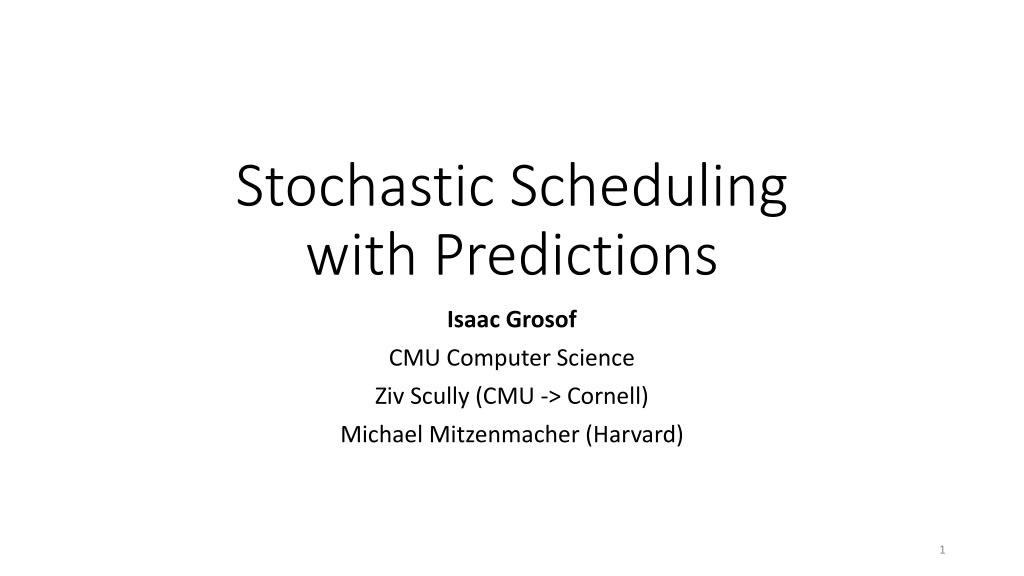
1. Stochastic Scheduling with Predictions Isaac Grosof CMU Computer Science Ziv Scully (CMU -> Cornell) Michael Mitzenmacher (Harvard) 1

2. Scheduling with Predictions Uniform Bounds for Scheduling with Job Size Estimates ITCS 2022 Response time T Goal: Minimize mean response time (E[T]) 2

3. Scheduling with Predictions Uniform Bounds for Scheduling with Job Size Estimates ITCS 2022 1.2 0.8 0.8 0.3 0.4 Response time T Goal: Minimize mean response time (E[T]) Known sizes: Shortest Remaining Processing Time (SRPT) is optimal Predicted sizes: ? 3

4. Stochastic Scheduling with Predictions Two ways to study: This talk Worst Case Analysis Stochastic Analysis Why stochastic analysis for scheduling? Overcomes worst-case barriers Challenging, subtle problems Reflects real world 4

5. Why Stochastic Arrivals? Worst case setting: General arrival sequence Size Time 5

6. Why Stochastic Arrivals? Worst case setting: General arrival sequence Real world: lots of independent arrival sequences Size Time 6

7. Why Stochastic Arrivals? Worst case setting: General arrival sequence Real world: lots of independent arrival sequences Size Time Approximation for large systems: Exponential interarrival times (Poisson) I.i.d. sizes 7

8. Example of Scheduling with Predictions 1 1 1 1.01 8

9. Example of Scheduling with Predictions 1 1 ALG: 3 jobs 1 1.01 0.01 0.01 0.01 0.01 9

10. Example of Scheduling with Predictions 1 1 ALG: 3 jobs OPT: 2 jobs 1 1.01 0.01 0.01 0.01 0.01 Tiny prediction error 3/2 competitive ratio Very unlikely in our stochastic model Goal: Tiny prediction error Near-perfect performance 10

11. Specific model Z Z Z Z Z Poisson( ) S S S S S Arrival process: Poisson( ) Size and predicted size i.i.d. from (?,?) ? [??,??] (S,Z) distribution chosen adversarially Scheduler does not know ?,?,?,? ? ?? ? ???? ? ?? ? ????? = Metric: 11

12. Performance Goals ? ?? ? ?????: Goals for ? ?? ? ?????= 1 Consistency: lim ?,? 1 ? ?? ? ????? ?? Graceful Degradation: ?,?, ? ? ?? ? ????? ? Robustness: ?,?, 12

13. Nave Scheduling Policy SRPT: Rank = ? ? Lower is better SRPT-E: z ? rank s z age z s Jobs uninterrupted when exceed prediction Lower bound: ? ????? ? ? If ? ?2= ,? ? = . In datacenter and webserver traces, ? ?2 very large 21 ?2?[?2] 13

14. SRPT with Checkmark SRPT-C: |z ?| rank z age z 2z ? ????? ? ? ????? SRPT-C is consistent: lim = 1 ?,? 1 First consistent policy! Not gracefully degrading: if ? <1 2,? ????? ? ? ????? unbounded. 14

15. SRPT with Bounce SRPT-B: min( z ? ,?) rank z age z 2z First policy to be consistent and gracefully degrading! 15

16. rank Results z age ? ????? ? ? ????? ? z 2z ??(?,?) 3 2?1 ? < 1 + 1 min 1,max 1 1 ?,1 where ? ?,? = 1 + ? 1 lim ?,? 1? ?,? = 1 (Consistency) ?,?, ? ?,? 3.5 (Graceful degradation) Robustness impossible, Gittins policy lower bound 16

17. Proof Methods SRPT-B: min( z ? ,?) SRPT-SE: z SRPT: ? ? s(? ?) rank ? ? ? ?,? s z z age s s z 2z Proof uses cutting-edge queueing theory: SOAP WINE ? ? ? Analysis of E[T] for rank-function policies ?? ? = ? ? = ?? ?2 0 17

18. SRPT-SE: z SRPT: ? ? s(? ?) SRPT-SE vs. SRPT ? ? s z r s s r-relevant work: ? ? = (?? ?)1{?? ? ?} Thm: SRPT minimizes ? ? :E WSRPTr E W?r ?,? ? ?r Thm: SRPT-SE nearly min. ? ? :E WSRPT SEr E W? ?,? ? ?r E WSRPT SEr E W???? ? ? ? WINE: ? ? =1 ?? ? 0 ? ????? ?? ? ?? ????? ?2 18

19. Zooming Out on Scheduling with Predictions Today: Unknown prediction distribution (?,?) Known prediction distribution: Single server solved by Gittins policy Multiserver: The Gittins Policy is Nearly Optimal in the M/G/k under Extremely General Conditions , [G., Scully, Harchol-Balter], SIGMETRICS 2021 Strategic predictions: Incentive Compatible Queues Without Money , [G., Mitzenmacher], arXiv 19

20. Stochastic Scheduling with Predictions igrosof@cmu.edu isaacg1.github.io ? ????? ? ? ????? rank SRPT-B: min( z ? ,?) lim ?,? 1 ? ????? ? ? ????? = 1 z 3.5? age ? z 2z 20