Multiprocessors Interconnection Networks
Multiprocessors Interconnection Networks
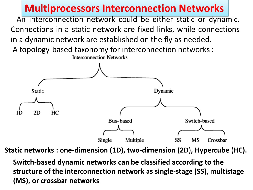
An interconnection network could be either static or dynamic.
Connections in a static network are fixed links, while connections
in a dynamic network are established on the fly as needed.
A topology-based taxonomy for interconnection networks :
Static networks : one-dimension (1D), two-dimension (2D), Hypercube (HC).
Switch-based dynamic networks can be classified according to the
structure of the interconnection network as single-stage (SS), multistage
(MS), or crossbar networks
Bus-Based Dynamic Interconnection Networks
1- Single Bus Systems
In its general form, such a system consists of
N
processors, each
having its own cache, connected by a shared bus. The use of local
caches reduces the processor–memory traffic. All processors
communicate with a single shared memory. The actual size is
determined by the traffic per processor and the bus bandwidth.
The single bus
network
complexity, measured in terms of the
number of buses used, is
O(1)
, while the
time
complexity,
measured in terms of the amount of input to output delay is
O(N)
.
2- Multiple Bus Systems
A multiple bus multiprocessor system uses several parallel buses to
interconnect multiple processors and multiple memory modules. A
number of connection schemes are possible in this case.
(a) -MBFBMC:
multiple bus with full bus–memory connection
(b) -MBSBMC:
multiple bus with single bus memory connection
(c) -MBPBMC:
multiple bus with partial bus–memory connection
(d) -MBCBMC:
multiple bus with class-based memory connection.
The multiple bus with full bus–memory connection has all memory
modules connected to all buses. The multiple bus with single bus–
memory connection has each memory module connected to a specific
bus. The multiple bus with partial bus–memory connection has each
memory module connected to a subset of buses. The multiple bus with
class-based memory connection has memory modules grouped into
classes whereby each class is connected to a specific subset of buses. A
class is just an arbitrary collection of memory modules. Illustrations of
these connection schemes for the case of N = 6 processors, M = 4
memory modules, and B = 4 buses as below:
One can characterize those connections using the number of connections
required and the load on each bus as shown in Table . In this table, k
represents the number of classes; g represents the number of buses per
group, and Mj represents the number of memory modules in class j.
TABLE of Characteristics of Multiple Bus Architectures
multiple bus multiprocessor organization offers a number of desirable
features such as high reliability and ease of incremental growth. A
single bus failure will leave (B-1) distinct fault-free paths between the
processors and the memory modules. On the other hand, when the
number of buses is less than the number of memory modules (or the
number of processors), bus contention is expected to increase.
Switch-Based Interconnection Networks
In this type of network, connections among processors
and memory modules are made using simple switches. Three
basic interconnection topologies exist: crossbar, single-stage, and
multistage.
1- Crossbar Networks
2- Single-Stage Networks
3- Multistage Networks
While the single bus can provide only a single connection, the crossbar
can provide simultaneous connections among all its inputs and all its
outputs. The crossbar contains a switching element (SE) at the
intersection of any two lines extended horizontally or vertically inside
the switch. For example the 8x8 crossbar network an SE (also called a
cross-point) is provided at each of the 64 SEs or (intersection points)
and the message delay to traverse from the input to the output is
constant, regardless of which input/output are communicating.
1- Crossbar Networks:-
The two possible settings of an SE in the crossbar (straight and
diagonal) .In general for an NxN crossbar, the network complexity,
measured in terms of the number of switching points, is O(N
2
) while
the time complexity, measured in terms of the input to output delay,
is O(1).
An 8x8 crossbar network
(a)
straight switch setting; (b) diagonal switch setting
2- Single-Stage Networks
The simplest switching element that can be used is the 2x2 switching
element (SE). With four possible settings
A well-known connection pattern for interconnecting the inputs(source)
and the outputs (destination)of a single-stage network is the Shuffle–
Exchange. Two operations are used. These can be defined using an m
bit-wise address pattern of the inputs, p
m-1
p
m-2
. . . p
1
p
0
, as follows:
If the number of inputs, for example, processors, in a single-stage IN is N
and the number of outputs, for example, memories, is N, the number of
SEs in a stage is N/2. The maximum length of a path from an input to an
output in the network, measured by the number of SEs along the path, is
log
2
N.
The network complexity of the single-stage interconnection
network is O(N) and the time complexity is O(N).
Example
In an 8-input single stage Shuffle–Exchange if the source is 0 (000)
and the destination is 6 (110), then the following is the required sequence of
Shuffle/ Exchange operations and circulation of data:
In addition to the shuffle and the exchange functions, there exist other
interconnection patterns. Among these are the Cube and the Plus-
Minus 2
i
(PM2I) networks.
The Cube Network
Consider a 3-bit
address (N = 8),
we have
C
2
(6) = 2,
C
1
(7) = 5
C
0
(4) = 5.
The Plus–Minus 2
i
(PM2I)
Network
The PM2I network consists of 2k interconnection functions defined as below:
For example, consider the case N = 8, PM2
+
1
(4) =4
+ 2
1
mod 8 = 6.
The PM2I network
for N =8
(a), PM2
+
0
for N = 8;
(b) PM2
+
1
for N =8;
(c) PM2
+
2
for N = 8.
T
h
e
B
u
t
t
e
r
f
l
y
F
u
n
c
t
i
o
n
T
h
e
i
n
t
e
r
c
o
n
n
e
c
t
i
o
n
p
a
t
t
e
r
n
u
s
e
d
i
n
t
h
e
b
u
t
t
e
r
f
l
y
n
e
t
w
o
r
k
i
s
d
e
f
i
n
e
d
a
s
f
o
l
l
o
w
s
:
C
o
n
s
i
d
e
r
a
3
-
b
i
t
a
d
d
r
e
s
s
(
N
=
8
)
,
t
h
e
f
o
l
l
o
w
i
n
g
i
s
t
h
e
b
u
t
t
e
r
f
l
y
m
a
p
p
i
n
g
:
Multistage Networks
The most undesirable single bus limitation that Multistage
interconnection networks (MINs ) is set to improve is the availability
of only one single path between the processors and the memory
modules. Such MINs provide a number of simultaneous paths
between the processors and the memory modules. A general MIN
consists of a number of stages each consisting of a set of 2x2
switching elements. Stages are connected to each other using Inter-
stage Connection (ISC) Pattern. These patterns may follow any of the
routing functions such as Shuffle–Exchange, Butterfly, Cube, and so
on. The settings of the SEs give a number of paths can be established
simultaneously. For example, the figure below shows how three
simultaneous paths connecting the three pairs of input/output 000
→101,101→011, and 110→010 can be established. It should be
noted that the interconnection pattern among stages follows the
shuffle operation. This network is known as the Shuffle–Exchange
network (SEN).as An example 8 x 8 (SEN).
The Banyan Network
The memory modules, is N, the number of MIN stages is log
2
N and the
number of SEs per stage is N/2, and hence the network complexity,
measured in terms of the total number of SEs is O(N x log
2
N). The time
complexity, measured by the number of SEs along the path from input to
output, is O(log
2
N). For example, in a 16x16 MIN, the length of the path
from input to output is 4. The total number of SEs in the network is usually
taken as a measure for the total area of the network. The total area of a
16x16 MIN is 32 SEs.
The Omega Network
A size N omega network consists of n (n=log
2
N single-stage) Shuffle–
Exchange networks. Each stage consists of a column of N=2, two-input
switching elements whose input is a shuffle connection
Number of Stages =
(Log
2
n)
Number of Switches per Stage =
(n/2),
Total Switches =
(n/2)Log
2
n
A commonly used multistage connection network is the
omega network
.
This network consists of log
p
stages, where
p
is the number of inputs
(processing nodes) and also the number of outputs (memory banks).
Each stage of the omega network consists of an interconnection pattern
that connects
p
inputs and
p
outputs; a link exists between input
i
and
output
j
if the following is true:
Equation 6.1 represents a left-rotation operation on the binary representation of
i
to obtain
j
. This interconnection pattern is called a
perfect shuffle
. Figure below
shows a perfect shuffle interconnection pattern for eight inputs and outputs. At
each stage of an omega network, a perfect shuffle interconnection pattern feeds
into a set of
p
/2 switches or switching nodes. It should be noted that the
interconnection pattern among stages follows the shuffle operation.
Equation 6.1
CPU 011 read From 110
Message Format
•
Module
It tell which memory to use.
•
Address
It specifies an address within a module
•
Opcode
Gives the operation, READ or WRITE
•
Value
Contain an operand.
Blockage in Multistage Interconnection Networks
A number of classification criteria exist for MINs. Among these
criteria is the criterion of blockage. According to this criterion, MINs
are classified as follows.
Blocking Networks
the concept of blocking network is that not all
possible here to make the input-output connections at the same time
as one path might block another. Examples of blocking networks
include Omega, Banyan, Shuffle–Exchange, the Data Manipulator, Flip,
N cube and Baseline.
Rearrangeable Networks:
Re-arrangeable networks are characterized
by the property that it
is always possible
to rearrange already
established connections in order to make allowance for other
connections to be established simultaneously. An example is Benes
network which support synchronous data permutation and a
synchronous inter-processor communication.
Non-blocking Networks
A non –blocking network is the network
which can handle all possible connections without blocking.
In the presence of a connection between input 101 and output 011, a
connection between input 100 and output 001 is not possible. This is
because the connection 101 to 011 uses the upper output of the third switch
from the top in the first stage. This same output will be needed by the
requested connection 100 to 001. This contention will lead to the inability
to satisfy the connection 100 to 001, that is, blocking. Notice however that
while connection 101 to 011 is established, the arrival of a request for a
connection such as 100 to 110 can be satisfied.
an example 8x8 Benes network. Two simultaneous connections are
shown established in the network. These are 110→100 and 010→110.
In the presence of the connection 110→100, it will not be possible to
establish the connection 101→001 unless the connection 110→100 is
rearranged as shown in part (b) of the figure.
The Clos is a well-known example of non-blocking networks. It
consists of
r1n1 x m input crossbar switches
(
r1
is the number of input
crossbars, m xn1 is the size of each input crossbar),
mr1 x r2 middle crossbar switches
(m is the number of middle
crossbars, and
r1 x r2
is the size of each middle crossbar),
r2m x n2 output crossbar switches
(
r2
is the number of output
crossbars and
m x n2
is the size of each output crossbar).
The Clos network is not blocking if the following inequality is satisfied
m ≥ n1+
n2 – 1
A three-stage Clos network is shown in Figure below . The network
has the following parameters: r1 = 4, n1 = 2, m = 4, r2 = 4, and n2 = 2.
The reader is encouraged to ascertain the non-blocking feature of the
network shown in Figure below by working out some example
simultaneous connections. For example show that in the presence of a
connection such as 110 to 010, any other connection will be possible.
Non-blocking Networks
In the realm of multiprocessors, interconnection networks play a crucial role. The distinction between static and dynamic networks lies in how connections are managed - fixed links versus on-the-fly establishment. Understanding this contrast is key in network design and performance optimization.

Download Presentation

Please find below an Image/Link to download the presentation.
The content on the website is provided AS IS for your information and personal use only. It may not be sold, licensed, or shared on other websites without obtaining consent from the author.If you encounter any issues during the download, it is possible that the publisher has removed the file from their server.
You are allowed to download the files provided on this website for personal or commercial use, subject to the condition that they are used lawfully. All files are the property of their respective owners.
The content on the website is provided AS IS for your information and personal use only. It may not be sold, licensed, or shared on other websites without obtaining consent from the author.
E N D
Presentation Transcript
Multiprocessors Interconnection Networks An interconnection network could be either static or dynamic. Connections in a static network are fixed links, while connections in a dynamic network are established on the fly as needed. A topology-based taxonomy for interconnection networks : Static networks : one-dimension (1D), two-dimension (2D), Hypercube (HC). Switch-based dynamic networks can be classified according to the structure of the interconnection network as single-stage (SS), multistage (MS), or crossbar networks
Bus-Based Dynamic Interconnection Networks 1- Single Bus Systems In its general form, such a system consists of N processors, each having its own cache, connected by a shared bus. The use of local caches reduces the processor memory traffic. All processors communicate with a single shared memory. The actual size is determined by the traffic per processor and the bus bandwidth. The single bus network complexity, measured in terms of the number of buses used, is O(1), while the time complexity, measured in terms of the amount of input to output delay is O(N).
2- Multiple Bus Systems A multiple bus multiprocessor system uses several parallel buses to interconnect multiple processors and multiple memory modules. A number of connection schemes are possible in this case. (a) -MBFBMC: multiple bus with full bus memory connection (b) -MBSBMC: multiple bus with single bus memory connection (c) -MBPBMC: multiple bus with partial bus memory connection (d) -MBCBMC: multiple bus with class-based memory connection. The multiple bus with full bus memory connection has all memory modules connected to all buses. The multiple bus with single bus memory connection has each memory module connected to a specific bus. The multiple bus with partial bus memory connection has each memory module connected to a subset of buses. The multiple bus with class-based memory connection has memory modules grouped into classes whereby each class is connected to a specific subset of buses. A class is just an arbitrary collection of memory modules. Illustrations of these connection schemes for the case of N = 6 processors, M = 4 memory modules, and B = 4 buses as below:
One can characterize those connections using the number of connections required and the load on each bus as shown in Table . In this table, k represents the number of classes; g represents the number of buses per group, and Mj represents the number of memory modules in class j. TABLE of Characteristics of Multiple Bus Architectures multiple bus multiprocessor organization offers a number of desirable features such as high reliability and ease of incremental growth. A single bus failure will leave (B-1) distinct fault-free paths between the processors and the memory modules. On the other hand, when the number of buses is less than the number of memory modules (or the number of processors), bus contention is expected to increase.
Switch-Based Interconnection Networks In this type of network, connections among processors and memory modules are made using simple switches. Three basic interconnection topologies exist: crossbar, single-stage, and multistage. 1- Crossbar Networks 2- Single-Stage Networks 3- Multistage Networks 1- Crossbar Networks:- While the single bus can provide only a single connection, the crossbar can provide simultaneous connections among all its inputs and all its outputs. The crossbar contains a switching element (SE) at the intersection of any two lines extended horizontally or vertically inside the switch. For example the 8x8 crossbar network an SE (also called a cross-point) is provided at each of the 64 SEs or (intersection points) and the message delay to traverse from the input to the output is constant, regardless of which input/output are communicating.
The two possible settings of an SE in the crossbar (straight and diagonal) .In general for an NxN crossbar, the network complexity, measured in terms of the number of switching points, is O(N2) while the time complexity, measured in terms of the input to output delay, is O(1). An 8x8 crossbar network (a) straight switch setting; (b) diagonal switch setting
2- Single-Stage Networks The simplest switching element that can be used is the 2x2 switching element (SE). With four possible settings A well-known connection pattern for interconnecting the inputs(source) and the outputs (destination)of a single-stage network is the Shuffle Exchange. Two operations are used. These can be defined using an m bit-wise address pattern of the inputs, pm-1pm-2 . . . p1p0, as follows: If the number of inputs, for example, processors, in a single-stage IN is N and the number of outputs, for example, memories, is N, the number of SEs in a stage is N/2. The maximum length of a path from an input to an output in the network, measured by the number of SEs along the path, is log2 N. The network complexity of the single-stage interconnection network is O(N) and the time complexity is O(N).
Example In an 8-input single stage ShuffleExchange if the source is 0 (000) and the destination is 6 (110), then the following is the required sequence of Shuffle/ Exchange operations and circulation of data: In addition to the shuffle and the exchange functions, there exist other interconnection patterns. Among these are the Cube and the Plus- Minus 2i(PM2I) networks. The Cube Network Consider a 3-bit address (N = 8), we have C2(6) = 2, C1(7) = 5 C0(4) = 5.
The PlusMinus 2i (PM2I)Network The PM2I network consists of 2k interconnection functions defined as below: For example, consider the case N = 8, PM2+1(4) =4 + 21 mod 8 = 6. The PM2I network for N =8 (a), PM2+0 for N = 8; (b) PM2+1 for N =8; (c) PM2+2 for N = 8.
The Butterfly Function The interconnection pattern used in the butterfly network is defined as follows: Consider a 3-bit address (N =8), the following is the butterfly mapping:
Multistage Networks The most undesirable single bus limitation that Multistage interconnection networks (MINs ) is set to improve is the availability of only one single path between the processors and the memory modules. Such MINs provide a number of simultaneous paths between the processors and the memory modules. A general MIN consists of a number of stages each consisting of a set of 2x2 switching elements. Stages are connected to each other using Inter- stage Connection (ISC) Pattern. These patterns may follow any of the routing functions such as Shuffle Exchange, Butterfly, Cube, and so on. The settings of the SEs give a number of paths can be established simultaneously. For example, the figure below shows how three simultaneous paths connecting the three pairs of input/output 000 101,101 011, and 110 010 can be established. It should be noted that the interconnection pattern among stages follows the shuffle operation. This network is known as the Shuffle Exchange network (SEN).as An example 8 x 8 (SEN).
The Banyan Network The memory modules, is N, the number of MIN stages is log2 N and the number of SEs per stage is N/2, and hence the network complexity, measured in terms of the total number of SEs is O(N x log2 N). The time complexity, measured by the number of SEs along the path from input to output, is O(log2 N). For example, in a 16x16 MIN, the length of the path from input to output is 4. The total number of SEs in the network is usually taken as a measure for the total area of the network. The total area of a 16x16 MIN is 32 SEs.
The Omega Network Number of Stages = (Log2n) Number of Switches per Stage = (n/2), Total Switches = (n/2)Log2n A size N omega network consists of n (n=log2 N single-stage) Shuffle Exchange networks. Each stage consists of a column of N=2, two-input switching elements whose input is a shuffle connection
A commonly used multistage connection network is the omega network. This network consists of log p stages, where p is the number of inputs (processing nodes) and also the number of outputs (memory banks). Each stage of the omega network consists of an interconnection pattern that connects p inputs and p outputs; a link exists between input i and output j if the following is true:
Equation 6.1 Equation 6.1 represents a left-rotation operation on the binary representation of i to obtain j. This interconnection pattern is called a perfect shuffle. Figure below shows a perfect shuffle interconnection pattern for eight inputs and outputs. At each stage of an omega network, a perfect shuffle interconnection pattern feeds into a set of p/2 switches or switching nodes. It should be noted that the interconnection pattern among stages follows the shuffle operation.
CPU 011 read From 110 Message Format Module It tell which memory to use. Address It specifies an address within a module Opcode Gives the operation, READ or WRITE Value Contain an operand.
Blockage in Multistage Interconnection Networks A number of classification criteria exist for MINs. Among these criteria is the criterion of blockage. According to this criterion, MINs are classified as follows. Blocking Networks the concept of blocking network is that not all possible here to make the input-output connections at the same time as one path might block another. Examples of blocking networks include Omega, Banyan, Shuffle Exchange, the Data Manipulator, Flip, N cube and Baseline. Rearrangeable Networks: Re-arrangeable networks are characterized by the property that it is always possible to rearrange already established connections in order to make allowance for other connections to be established simultaneously. An example is Benes network which support synchronous data permutation and a synchronous inter-processor communication. Non-blocking Networks A non blocking network is the network which can handle all possible connections without blocking.
In the presence of a connection between input 101 and output 011, a connection between input 100 and output 001 is not possible. This is because the connection 101 to 011 uses the upper output of the third switch from the top in the first stage. This same output will be needed by the requested connection 100 to 001. This contention will lead to the inability to satisfy the connection 100 to 001, that is, blocking. Notice however that while connection 101 to 011 is established, the arrival of a request for a connection such as 100 to 110 can be satisfied.
In the presence of a connection between input 101 and output 011, a connection between input 100 and output 001 is not possible. This is because the connection 101 to 011 uses the upper output of the third switch from the top in the first stage. This same output will be needed by the requested connection 100 to 001. This contention will lead to the inability to satisfy the connection 100 to 001, that is, blocking. Notice however that while connection 101 to 011 is established, the arrival of a request for a connection such as 100 to 110 can be satisfied.
an example 8x8 Benes network. Two simultaneous connections are shown established in the network. These are 110 100 and 010 110. In the presence of the connection 110 100, it will not be possible to establish the connection 101 001 unless the connection 110 100 is rearranged as shown in part (b) of the figure.
Non-blocking Networks The Clos is a well-known example of non-blocking networks. It consists of r1n1 x m input crossbar switches (r1 is the number of input crossbars, m xn1 is the size of each input crossbar), mr1 x r2 middle crossbar switches (m is the number of middle crossbars, and r1 x r2 is the size of each middle crossbar), r2m x n2 output crossbar switches (r2 is the number of output crossbars and m x n2 is the size of each output crossbar). The Clos network is not blocking if the following inequality is satisfied m n1+ n2 1 A three-stage Clos network is shown in Figure below . The network has the following parameters: r1 = 4, n1 = 2, m = 4, r2 = 4, and n2 = 2. The reader is encouraged to ascertain the non-blocking feature of the network shown in Figure below by working out some example simultaneous connections. For example show that in the presence of a connection such as 110 to 010, any other connection will be possible.


Network")