Lecture 8 Valuation Models for Stock Prices


L
e
c
t
u
r
e
8
V
a
l
u
a
t
i
o
n
M
o
d
e
l
s
f
o
r
S
t
o
c
k
P
r
i
c
e
s
n
Cash Flow Models of Equity Valuation.
n
Dividend Discount Models
n
Accrual Discount Models
n
Determining the Value Drivers
n
Cases in Valuation Model Analysis
n
Reading: SAIS, sec. 8.1, 8.2 and 8.3 and
Case Downloads from the
Class Webpage (see last slides in this lecture)

C
o
n
n
e
c
t
i
o
n
t
o
F
i
n
a
l
E
x
a
m
Q
u
e
s
t
i
o
n
ii)
“The search for the 'correct' way to value common stocks, or even one that works,
has occupied a huge amount of effort over a long period of time....the implementation
of a system to selectively value or select common stocks is a difficult task. This is a
task that a valuation model purports to
accomplish.”
Describe the
discounted dividend
cash flow valuation models conventionally used
to analyse common stocks. How do these models differ from valuation models that
discount cash flows other than dividends? What are some important limitations of
using accounting data to implement
discounted cash flow valuation?
It is commonplace to hear that discounted cash flow (DCF) models are the
appropriate way to value common stocks – in the context of value investing,
DCF has been proposed as the way to estimate ‘intrinsic value’. This lecture
covers these models and the connection to using accounting data for stock
valuation.
It is doubtful that such models can do any more than provide some structure
to a stock valuation. As the quote recognizes, stock valuation is ‘a difficult
task’ –
too difficult in many cases for a formula to capture
.

B
a
s
i
c
s
o
f
D
i
s
c
o
u
n
t
e
d
C
a
s
h
F
l
o
w
V
a
l
u
a
t
i
o
n
n
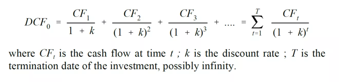
The basic models can be specified as:
Key issues:
What is the relevant cash flow variable?
What is the terminal cash flow?
How to get the discount rate?
NOTE: For an equity security all of the rhs variables are
unknown on the valuation date
t =
0.
H
i
s
t
o
r
y
o
f
D
i
s
c
o
u
n
t
e
d
C
a
s
h
F
l
o
w
(
D
C
F
)
M
o
d
e
l
s
n
Origins of
DCF
models for security valuation can be
found in John Burr Williams
The Theory of
Investment Value
(1938).
u
The present value for a business or a security,
such as a stock or bond, can be determined by
discounting the future stream of expected cash
inflows minus expected cash outflows at the
appropriate rate of interest.
n
The basic
DCF
model was adapted and expanded in
the
DDM
of Gordon (1962)
u
valuation of companies in regulated industries was a
central concern.
u
the constant growth version of the discounted dividend
model is often referred to as the ‘Gordon growth model’
W
h
o
w
a
s
J
o
h
n
B
u
r
r
W
i
l
l
i
a
m
s
(
1
9
0
0
-
1
9
8
9
)
?
n
W
i
l
l
i
a
m
s
i
s
c
r
e
d
i
t
e
d
w
i
t
h
b
e
i
n
g
a
n
e
a
r
l
y
p
r
o
p
o
n
e
n
t
o
f
u
s
i
n
g
d
i
s
c
o
u
n
t
e
d
c
a
s
h
f
l
o
w
t
o
e
s
t
i
m
a
t
e
t
h
e
‘
i
n
t
r
i
n
s
i
c
v
a
l
u
e
’
o
f
a
s
t
o
c
k
.
n
This represented a more theoretical
and mathematical approach to
‘intrinsic value’ than the relatively
heuristic notions previously available.
n
Williams was a long time student at
Harvard and the
Theory of
Investment Value
was his Harvard
PhD thesis in Economics
n
Williams worked as a securities
analyst and sometime professor.
J
.
B
.
W
i
l
l
i
a
m
s
D
C
F
m
o
d
e
l
w
a
s
n
o
t
n
e
w
.
P
r
e
v
i
o
u
s
w
r
i
t
e
r
s
s
u
c
h
a
s
M
a
c
a
u
l
a
y
(
1
9
3
8
)
q
u
e
s
t
i
o
n
e
d
t
h
e
a
p
p
l
i
c
a
t
i
o
n
o
f
D
C
F
t
o
v
a
l
u
e
c
o
m
m
o
n
s
t
o
c
k
s
T
h
e
‘
a
s
s
u
m
p
t
i
o
n
o
f
p
a
y
m
e
n
t
’
,
w
h
i
c
h
m
u
s
t
b
e
m
a
d
e
b
e
f
o
r
e
t
h
e
p
r
o
m
i
s
e
d
o
r
‘
h
y
p
o
t
h
e
t
i
c
a
l
’
y
i
e
l
d
o
f
a
b
o
n
d
c
a
n
b
e
c
a
l
c
u
l
a
t
e
d
.
.
.
m
a
y
,
a
s
w
e
h
a
v
e
s
e
e
n
,
b
e
a
m
e
r
e
m
a
t
h
e
m
a
t
i
c
a
l
f
i
c
t
i
o
n
f
o
r
a
l
l
e
x
c
e
p
t
t
h
e
h
i
g
h
e
s
t
g
r
a
d
e
o
f
b
o
n
d
s
.
B
u
t
,
f
o
r
c
o
m
m
o
n
s
t
o
c
k
s
i
t
i
s
n
o
t
o
n
l
y
a
m
a
t
h
e
m
a
t
i
c
a
l
f
i
c
t
i
o
n
b
u
t
a
l
s
o
a
n
e
c
o
n
o
m
i
c
a
b
s
u
r
d
i
t
y
.
E
v
e
n
i
f
t
h
e
c
h
a
n
c
e
t
h
a
t
t
h
e
p
r
o
m
i
s
e
s
c
o
n
t
a
i
n
e
d
i
n
a
b
o
n
d
w
i
l
l
b
e
k
e
p
t
i
s
n
e
g
l
i
g
i
b
l
y
s
m
a
l
l
t
h
a
t
t
h
e
p
r
o
m
i
s
e
s
a
r
e
l
i
t
t
l
e
m
o
r
e
t
h
a
n
m
e
r
e
w
o
r
d
s
,
t
h
e
y
a
r
e
a
t
l
e
a
s
t
d
e
f
i
n
i
t
e
w
o
r
d
s
a
n
d
,
a
s
s
u
c
h
,
c
a
n
s
t
a
n
d
t
h
e
s
t
r
a
i
n
o
f
m
a
t
h
e
m
a
t
i
c
a
l
m
a
n
i
p
u
l
a
t
i
o
n
.
M
a
c
a
u
l
a
y
(
1
9
3
8
)
T
h
e
M
o
v
e
m
e
n
t
o
f
I
n
t
e
r
e
s
t
R
a
t
e
s
,
B
o
n
d
s
,
Y
i
e
l
d
s
a
n
d
S
t
o
c
k
P
r
i
c
e
s
i
n
t
h
e
U
n
i
t
e
d
S
t
a
t
e
s
s
i
n
c
e
1
8
6
5
w
a
s
a
m
o
n
u
m
e
n
t
a
l
N
B
E
R
s
t
u
d
y
.
O
n
k
=
g
i
n
t
h
e
G
o
r
d
o
n
D
D
M
m
o
d
e
l
,
M
a
c
a
u
l
a
y
o
b
s
e
r
v
e
d
:
n
I
f
…
t
h
e
d
i
v
i
d
e
n
d
p
a
y
m
e
n
t
s
w
e
r
e
t
o
i
n
c
r
e
a
s
e
i
n
g
e
o
m
e
t
r
i
c
p
r
o
g
r
e
s
s
i
o
n
…
O
n
e
o
f
t
h
e
s
t
r
a
n
g
e
s
t
r
a
t
i
o
n
a
l
i
z
a
t
i
o
n
s
o
f
u
n
e
n
d
i
n
g
p
r
i
c
e
r
i
s
e
t
h
a
t
a
p
p
e
a
r
e
d
i
n
t
h
e
m
o
n
t
h
s
i
m
m
e
d
i
a
t
e
l
y
p
r
e
c
e
d
i
n
g
t
h
e
s
t
o
c
k
m
a
r
k
e
t
c
u
l
m
i
n
a
t
i
o
n
o
f
1
9
2
9
w
a
s
e
v
o
l
v
e
d
b
y
a
W
a
l
l
S
t
r
e
e
t
e
c
o
n
o
m
i
s
t
.
H
e
p
r
e
s
e
n
t
e
d
t
o
t
h
e
d
i
r
e
c
t
o
r
s
o
f
t
h
e
i
n
v
e
s
t
m
e
n
t
t
r
u
s
t
…
s
t
a
t
i
s
t
i
c
a
l
e
v
i
d
e
n
c
e
t
h
a
t
t
h
e
w
e
a
l
t
h
o
f
t
h
e
c
o
u
n
t
r
y
i
n
c
r
e
a
s
e
d
i
n
t
h
e
l
o
n
g
r
u
n
a
b
o
u
t
3
p
e
r
c
e
n
t
p
e
r
a
n
n
u
m
.
H
e
t
h
e
n
a
r
g
u
e
d
t
h
a
t
c
o
r
p
o
r
a
t
i
o
n
s
a
s
a
c
l
a
s
s
s
h
o
u
l
d
b
e
e
x
p
e
c
t
e
d
t
o
s
h
a
r
e
i
n
t
h
i
s
g
r
o
w
t
h
a
t
t
h
i
s
r
a
t
e
a
n
d
h
e
n
c
e
t
h
a
t
t
h
e
i
r
d
i
v
i
d
e
n
d
s
s
h
o
u
l
d
b
e
e
x
p
e
c
t
e
d
,
o
v
e
r
t
h
e
l
o
n
g
r
u
n
,
t
o
i
n
c
r
e
a
s
e
a
t
l
e
a
s
t
3
p
e
r
c
e
n
t
p
e
r
a
n
n
u
m
;
t
h
a
t
i
s
t
o
s
a
y
i
n
s
u
c
h
a
s
e
r
i
e
s
a
s
$
4
.
1
2
,
$
4
.
2
4
,
$
4
.
3
7
,
e
t
c
.
,
o
r
$
4
(
1
.
0
3
)
,
$
4
(
1
.
0
3
)
2
,
$
4
(
1
.
0
3
)
3
,
e
t
c
.
H
e
t
h
e
n
s
u
g
g
e
s
t
e
d
t
h
a
t
…
t
h
e
s
e
f
u
t
u
r
e
d
i
v
i
d
e
n
d
s
w
o
u
l
d
e
v
e
n
t
u
a
l
l
y
b
e
d
i
s
c
o
u
n
t
e
d
a
t
a
r
a
t
e
t
h
a
t
w
o
u
l
d
n
o
t
e
x
c
e
e
d
3
p
e
r
c
e
n
t
p
e
r
a
n
n
u
m
.
B
u
t
,
h
e
c
o
n
t
i
n
u
e
d
,
i
f
d
i
s
t
a
n
t
e
n
o
u
g
h
p
a
y
m
e
n
t
s
w
e
r
e
a
s
s
u
m
e
d
,
d
i
s
c
o
u
n
t
i
n
g
t
h
e
m
a
t
t
h
i
s
r
a
t
e
w
o
u
l
d
g
i
v
e
v
e
r
y
h
i
g
h
p
r
i
c
e
s
f
o
r
t
h
e
s
t
o
c
k
s
.
T
h
e
s
u
g
g
e
s
t
i
o
n
w
a
s
e
v
e
n
m
a
d
e
t
h
a
t
,
a
s
t
h
e
r
e
s
e
e
m
e
d
t
o
b
e
n
o
n
e
c
e
s
s
a
r
y
t
i
m
e
l
i
m
i
t
t
o
t
h
e
3
p
e
r
c
e
n
t
r
a
t
e
o
f
g
r
o
w
t
h
i
n
w
e
a
l
t
h
,
t
h
e
r
e
s
h
o
u
l
d
l
o
g
i
c
a
l
l
y
b
e
n
o
‘
c
e
i
l
i
n
g
’
w
h
a
t
e
v
e
r
f
o
r
s
t
o
c
k
p
r
i
c
e
s
.
T
h
e
p
h
a
n
t
a
s
y
w
a
s
s
t
r
a
n
g
e
l
y
r
e
m
i
n
i
s
c
e
n
t
o
f
t
h
e
P
e
t
e
r
s
b
u
r
g
P
a
r
a
d
o
x
i
n
t
h
e
m
a
t
h
e
m
a
t
i
c
a
l
t
h
e
o
r
y
o
f
p
r
o
b
a
b
i
l
i
t
y
.
N
a
r
r
o
w
v
s
.
B
r
o
a
d
D
i
v
i
d
e
n
d
s
n
Initial conception of the dividend
DCF
models were
developed for high cash payout securities
u
Gordon focused on US utility stocks where the cash payout was
determined by state/federal rate setting bodies that set utility rates
for private companies
n
More recently, share buyback programs have been
replacing high cash payout
u
narrow dividends
are just cash dividend payout while
broad
dividends
include both buybacks and cash dividends
n
See three files in 417_lecture8.zip on growth of share
repurchases
N
a
r
r
o
w
a
n
d
B
r
o
a
d
D
i
v
i
d
e
n
d
s
f
o
r
P
f
i
z
e
r
(
f
r
o
m
1
0
-
K
)
B
a
s
i
c
D
C
F
m
o
d
e
l
:
T
h
e
D
D
M
n
Dividend Discount Model (
DDM):
Assume that the future
is known with certainty and that perfect market
assumptions apply.
u
No taxes and the term structure of discount rates is flat.
u
Assumes dividends are source of security cash flow
n
Assume that the stock to be valued is purchased at price
P(0)
and held for one period and then sold, the dividend
to be received in the next period is
Div(1)
) and the price
received from selling the stock is
P(1)
S
o
l
v
i
n
g
f
o
r
t
h
e
I
n
f
i
n
i
t
e
H
o
r
i
z
o
n
D
D
M
n
Notice the essential role of a simplified firm with ‘clean
surplus’ – no share repurchases, only dividends
n
Accounting for randomness in the future cash flows by
taking expectations conditional on information
available at
t=0
, the infinite horizon
DDM
is derived by
making a progressive substitution for prices:
A
p
p
l
y
i
n
g
t
h
e
D
D
M
:
P
r
e
f
e
r
r
e
d
S
t
o
c
k
V
a
l
u
a
t
i
o
n
n
Preferred Stocks
u
Rationales for preferred stock issuance
F
Role of Basel III for banks
F
Debt surrogates for corporations
•
Low credits and non-bank financials
n
Assume that
Div(t)
is fixed at
Div*
(
g = 0
)
u
Apply the perpetual pricing model
F
P(t) = Div* / k
u
Valuation for preferred shares involves comparison of the
dividend yield (similar to traditional yield spread analysis)
P
r
e
f
e
r
r
e
d
S
h
a
r
e
F
e
a
t
u
r
e
s
n
Fixed rate vs. Rate Reset
u
The reset rate can vary according to the length of time between
reset dates and the reference rate used for the reset
F
See Enbridge Examples
see CIBC ‘Canadian preferred shares’ report in
link to CIBC report on class webpage
F
www.prefinfo.com
(Hymas Investments) also has details of Cdn. Pref. shares
n
Retractable vs. Redeemable
u
Redeemable preferred shares, also known as callable preferred
shares, allows the issuer to buy back the (perpetual) preferred
stock at a fixed (call) price
F
Terms and conditions depend on the prospectus
u
Retractable preferred shares are issued with a maturity date when the
company can force the shareholders to redeem shares for a fixed
payment
F
Terms and conditions depend on the prospectus, the retraction may be an
exchange for common shares (not necessarily a cash price).
T
h
e
G
o
r
d
o
n
G
r
o
w
t
h
M
o
d
e
l
T
h
e
G
o
r
d
o
n
g
r
o
w
t
h
m
o
d
e
l
(
g
r
o
w
i
n
g
p
e
r
p
e
t
u
i
t
y
)
u
Assume the dividend changes over time according to the
assumption:
D(t+1) = D(t)(1 + g)
, where
g
is the assumed
constant growth rate in dividends.
E
x
a
m
p
l
e
s
o
f
A
p
p
l
y
i
n
g
t
h
e
F
o
r
m
u
l
a
n
SAIS, p.428-33, examines examples from
Damodaran (1994)
u
How is
k
estimated?
u
How is
g
estimated?
u
How is
D(1)
estimated?
u
What types of companies are examined?
n
Exercise: use Gordon model to value BUD,
GE and BCE
F
r
o
m
D
i
v
i
d
e
n
d
s
t
o
E
a
r
n
i
n
g
s
n
Dividends are problematic as a model for determining
stock prices as the limited variation in dividend payout
does not correspond to the substantial variation in stock
prices
transition to an earnings model
u
A
s
s
u
m
e
c
o
n
s
t
a
n
t
d
i
v
i
d
e
n
d
p
a
y
o
u
t
b
E
(
t
)
=
D
i
v
(
t
)
u
It follows that the constant dividend payout of the Gordon
model translates to earnings
F
b E(t+1) = Div(t+1) = Div(t) (1+g) = b E(t) (1+g)
F
Constant dividend growth with constant dividend payout
translates the substitution of earnings (which has more
substantial variation than dividends) in the Gordon Growth
model
P(0) = (b E(1)) / (k - g)
u
Damodaran estimates
k
using CAPM and
g
from past growth
rates
D
a
m
o
d
a
r
a
n
o
n
S
i
m
p
l
i
f
i
e
d
D
D
M
V
a
l
u
a
t
i
o
n
:
S
u
b
s
t
i
t
u
t
i
n
g
E
a
r
n
i
n
g
s
g
f
o
r
D
i
v
i
d
e
n
d
s
g
C
a
l
c
u
l
a
t
i
n
g
t
h
e
g
a
n
d
k
n
Estimating
g
by converting the problematic dividend
growth assumption to earnings growth requires
assuming a constant dividend payout ratio (
b
)
F
Damodaran estimates the
g
from the previous 5 years of
earnings
more realistic to take use the observed stock
price and use the formula to provide an implied growth rate
estimate
this can be used to interpret
P/E
F
Earnings are an accrual measure that might not represent
the underlying cash flows
possible to interpret
b
as a
broad dividend
F
How to interpret g
?
n
Estimating
k
using the
CAPM
requires
R
F
as the long
term bond rate, Damodaran estimates
β
(somehow?)
with geometric equity risk premium (
E[R
M
] –
R
F
)
estimated from 1925 to 1992
u
Is this the best way to get k?
T
w
o
m
o
r
e
D
a
m
o
d
a
r
a
n
E
x
a
m
p
l
e
s
:
E
x
x
o
n
,
D
r
e
s
d
n
e
r
Using Accruals for the Cash Flow: The
Residual Income Model
n
T
h
i
s
m
o
d
e
l
e
x
p
l
o
i
t
s
t
h
e
c
l
e
a
n
s
u
r
p
l
u
s
r
e
l
a
t
i
o
n
s
h
i
p
:
u
BV(t) = BV(t-1) + E(t) - D(t) = BV(t-1) + RE(t)
F
D(t) = E(t) –
Δ
BV
E(t) = D(t) + RE(t)
u
Clean surplus does not apply with share repurchases
or other manipulations of the equity account
n
The clean surplus equation is substituted into the
general DCF model to obtain
(AE
is ‘abnormal
earnings’, i.e., return on equity in excess of cost of
capital)
:
S
o
m
e
B
a
s
i
c
R
e
s
i
d
u
a
l
I
n
c
o
m
e
C
a
l
c
u
l
a
t
i
o
n
s
n
ROE
(
t
) =
E
(
t
) /
BV(t-1)
u
ROE
(return on equity) is an accrual measure
F
This is not a cash measure
n
k =
Δ
BV /
BV(t-1)
u
This is an interpretation for
k
that differs from the
CAPM
interpretation of the Gordon
DDM
n
‘Return on equity in excess of cost of capital’
interpretation of the residual income model needs to
be in an accounting, not economic, sense
I
n
t
e
r
p
r
e
t
i
n
g
R
e
t
u
r
n
o
n
E
q
u
i
t
y
n
Examine the numerator of the residual income model
u
(ROE(t) – k) BV(t-1)
F
This variable depends on the accrual relationship between
earnings and the change in book value
importance of clean
surplus
n
The
ROE
can be expressed in value driver format (Table 8.10,
p.467):
P
/
B
V
,
R
O
E
a
n
d
P
/
E
n
Conventional measures of relative valuation
are Price to Book Value (
P/BV
), Price to
Earnings (
P/E
) and Return on Equity (
ROE
)
u
Given any two the other is given
n
Assume Net Income and Earnings are the
same:
u
ROE
=
E / BV
u
P/E = (P / BV) ÷ (E / BV
)
F
This holds for aggregate and per share values
K
e
y
S
t
a
t
i
s
t
i
c
s
f
r
o
m
B
l
o
o
m
b
e
r
g
f
o
r
F
a
c
e
b
o
o
k
(
2
4
/
8
/
1
8
)
Different Forms of the P/E Ratio
n
The
P/E
ratio is a key valuation measure for practicing
security analysts
n
Letting
b
represent the dividend payout ratio (
Div(t) /
E(t)
), i.e.,
b E(t) = Div(t),
in the Gordon model the
P/E
ratio can be solved as:
n
Observe what the
P/E
is when
g =
0 (no growth) and
b =
1 (full earnings payout to dividends)
I
n
t
e
r
p
r
e
t
i
n
g
t
h
e
P
/
E
r
a
t
i
o
n
For a preferred stock
E = Div., b =
1,
g =
0
u
It follows that
P/E
= 1/
k*
this
k*
provides a low bound for
the
k
associated with common stock
n
Consider a stock that may or may not pay narrow dividends
(
ND
) and needs to allocate a constant fraction of cash flow to
sustain the growth of earnings (or alternatively, cash from
operations) at
g
and returns the remainder (
BD
) to
shareholders (as share buybacks, dividends, debt paydown,
increased asset purchases to fund increased future
g
)
u
To make sense of this
BDDM
version, i.e.,
k > g,
the
observed
P/E
implies
k
from the CAPM imposes an implied
estimate about the
E[R
i
]
and
β
for that stock
u
E.g., b
= .8
P/E
= 35
g =
10%
k = 12.5%
u
Increasing
g =
25%
k = 27.5%
S
c
e
n
a
r
i
o
s
f
o
r
k
i
n
B
D
D
M
g
i
v
e
n
g
&
b
&
P
/
E
*
P/E
5
20
50
b
.8
g
= .25
k = 45%
k = 30%
k = 27%
g
= .05
k = 22%
k = 9.2%
k = 6.7%
g = -.05
k = 10%
k = -1.2%
k = -3.5%
b
.5
g
= .25
k = 37.5%
k = 28%
k = 26%
g
= .05
k = 15.5%
k = 7.6%
k = 6.1%
g = -.05
k = 4.5%
k = -2.6%
k = -4%
b
.2
g
= .25
k = 30%
k = 26.3%
k = 25.5%
g
= .05
k = 9.2%
k = 6.1%
k = 5.4%
g = -.05
k = -1.2%
k = -4%
k = -4.6%
b
-.05
g
= .25
k = 23.8%
k = 24.7%
k = 24.9%
g
= .05
k = 4%
k = 4.7%
k = 4.9%
g = -.05
k = -5.9%
k = -5.2%
k = -5.1%
* What happens as b
0? (k
g why?)
P/E Ratio for the AE Model
n
The Residual Income Model can also be solved for a
P/E
ratio (after some manipulation)
n
Recalling that the definition for
AE(t)
requires,
k BV(t-1) =
E(t) - AE(t):
T
h
e
P
E
G
R
a
t
i
o
T
h
e
“
P
E
G
”
r
a
t
i
o
,
o
r
P
/
E
t
o
g
r
o
w
t
h
r
a
t
e
r
a
t
i
o
:
u
sometimes used as a crude rule of thumb to
determine under/over valuation for a common
stock.
F
For example, if the PEG ratio is less than one then
the stock is undervalued because the ‘cost of
growth’ as measured by the
P/E
is less than the
actual growth.
F
Problems with the PEG
based on accrual #
(earnings) and does not investigate sources of and
future prospects for growth
In terms of the
AE
model:
E
a
r
n
i
n
g
s
,
F
r
e
e
C
a
s
h
F
l
o
w
a
n
d
E
V
A
n
W
h
a
t
i
s
t
h
e
a
p
p
r
o
p
r
i
a
t
e
‘
c
a
s
h
f
l
o
w
’
t
o
d
i
s
c
o
u
n
t
i
n
t
h
e
D
C
F
m
o
d
e
l
?
u
‘
e
c
o
n
o
m
i
c
f
r
e
e
c
a
s
h
f
l
o
w
’
(
B
u
f
f
e
t
t
)
u
n
e
t
c
a
s
h
f
l
o
w
u
f
r
e
e
c
a
s
h
f
l
o
w
u
E
V
A
n
Higgins (1998, p.19) observes:
u
“So many conflicting definitions of cash flow exist
today that the term has almost lost meaning”
F
r
e
e
C
a
s
h
F
l
o
w
t
o
E
q
u
i
t
y
M
o
d
e
l
n
The free cash flow to equity model (
FCFE
) aims to measure the
return to equity above the amount required to: maintain existing
production levels; or, alternatively, to keep the firm on a particular
growth path.
u
Adjustments for payment to debt can create conceptual
problems
u
As with PEG,
FCFE
is an accrual number; Difficult to estimate future
values of
FCFE
n
Much the same manipulations as for the models using dividends can
be applied to this model (see sec. 8.3):
F
r
e
e
C
a
s
h
F
l
o
w
(
F
C
F
)
,
A
N
o
n
-
G
A
A
P
m
e
a
s
u
r
e
n
Various methods are suggested for
FCF
u
Free Cash Flow to the Firm (
FCFF
)
u
Free Cash Flow to Equity (
FCFE
)
u
Could be calculated from Income Statement or Cash Flow
Statement
n
Basic Idea is to provide a measure of Economic ‘Profit’
n
‘Simple
FCFF
’, determined from the Cash Flow
Statement:
FCFF = CFO – Cap. Ex.
n
‘Adjusted Simple
FCFF’: Simple FCFF – Div.
I
n
t
e
r
P
i
p
e
l
i
n
e
,
A
n
n
u
a
l
R
e
p
o
r
t
2
0
1
7
O
t
h
e
r
S
u
g
g
e
s
t
i
o
n
s
f
o
r
F
C
F
n
FCFF = EBIT(1 - Tax rate) + Depreciation -
Capital Expenditures ±
Δ
Net Working Capital
u
Mix of Income Statement and Cash Flow Statement and
Balance Sheet
n
FCFE = Net Income + Depreciation - Capital
expenditures
-
Δ
Net Working Capital
-
Debt
principal repayments + Proceeds of New Debt
Issues
u
Calculations from Cash Flow Statement
n
Note the potentially important impact of adjustments to Debt on
FCFE
W
h
a
t
i
s
w
o
r
k
i
n
g
c
a
p
i
t
a
l
?
n
Working Capital (WC) is a Balance Sheet Item
Working Capital = Current Assets – Current Liabilities
WC is often interpreted as a liquidity measure
Key Current Assets usually are
Cash and Marketable Securities
Inventories
Accounts Receivable
Key Current Liabilities usually are
Accounts payable
Short Term Borrowing
Accrued Liabilities
W
h
a
t
i
s
a
V
a
l
u
e
D
r
i
v
e
r
?
n
For equity securities, the key part of the
DCF
valuation is the
determining the numerator
n
A
v
a
l
u
e
d
r
i
v
e
r
i
s
a
f
a
c
t
o
r
t
h
a
t
h
a
s
a
s
i
g
n
i
f
i
c
a
n
t
i
m
p
a
c
t
o
n
t
h
e
l
e
v
e
l
a
n
d
c
h
a
n
g
e
o
f
t
h
e
c
a
s
h
f
l
o
w
t
h
a
t
d
r
i
v
e
s
e
q
u
i
t
y
s
e
c
u
r
i
t
y
v
a
l
u
e
.
u
Value drivers are essential items that need to be
identified in constructing the ‘story’ about a company,
e.g., Apple and iPhone demand
n
Two key dimensions to value drivers:
u
profitability
u
growth
T
h
e
S
t
o
r
y
:
C
O
S
S
y
n
c
r
u
d
e
V
a
l
u
a
t
i
o
n
n
C
a
n
a
d
i
a
n
O
i
l
S
a
n
d
s
(
C
O
S
.
U
N
)
w
a
s
a
u
n
i
t
t
r
u
s
t
w
i
t
h
o
w
n
e
r
s
h
i
p
i
n
S
y
n
c
r
u
d
e
a
s
t
h
e
s
o
l
e
i
n
c
o
m
e
p
r
o
d
u
c
i
n
g
a
s
s
e
t
.
T
h
e
c
o
m
p
a
n
y
w
a
s
f
o
r
m
e
d
i
n
2
0
0
1
b
y
t
h
e
m
e
r
g
e
r
o
f
t
w
o
p
r
e
v
i
o
u
s
e
n
t
i
t
i
e
s
r
e
s
u
l
t
i
n
g
i
n
a
n
o
n
-
o
p
e
r
a
t
i
n
g
e
n
t
i
t
y
w
i
t
h
2
1
.
7
%
o
w
n
e
r
s
h
i
p
o
f
t
h
e
S
y
n
c
r
u
d
e
o
i
l
s
a
n
d
s
p
r
o
j
e
c
t
.
n
The Syncrude oil sands project involves surface mining of
oil with an alternative technology
n
In Feb. 2003 COS announced the intention to buy 10% of
Syncrude from Encana
u
Problem to assess whether fair value was paid for the
purchase
n
COS was purchased by Suncor in 2016
u
Suncor was one of the partners in the Syncrude project
W
h
a
t
i
s
a
‘
u
n
i
t
t
r
u
s
t
’
?
n
Common stocks arising from limited liability corporations
(LLC) are one of a number of different methods of creating
tradeable equity claims
u
Other methods include limited liability partnerships (LLP) and
limited corporations (LC)
u
Key point: Different forms of organization have
different tax
implications
u
In the LLC taxes on profits are paid the firm level with dividend
payments receiving favorable personal income tax treatment
n
A unit trust has a ‘flow through’ tax structure where the
payment to unit holders are treated like debt payments,
deductible at the firm level, with tax implications passing to
unit holders at full personal income tax rates
F
Unit trusts have theoretical unlimited liability
F
Tax treatment is similar to limited partners in LLP
P
r
o
b
l
e
m
s
?
A
D
C
F
f
o
r
C
a
n
a
d
i
a
n
O
i
l
S
a
n
d
s
n
The DCF was conducted by a professional engineering firm to value
the initial COS unit trust issue. A number were required: SSB prices
off WTI (US$), gas is used to heat the slurry
R
e
s
u
l
t
o
f
t
h
e
D
C
F
w
i
t
h
e
s
c
a
l
a
t
i
n
g
c
o
s
t
s
a
n
d
p
r
i
c
e
s
C
o
m
p
a
r
e
t
h
e
p
r
e
d
i
c
t
i
o
n
s
w
i
t
h
a
c
t
u
a
l
f
u
t
u
r
e
p
r
i
c
e
p
e
r
f
o
r
m
a
n
c
e
Oil price
prediction
here
C
a
l
c
u
l
a
t
i
n
g
t
h
e
D
C
F
f
o
r
t
h
e
C
o
m
b
i
n
e
d
e
n
t
i
t
i
e
s
n
Even a relatively simple valuation scenario associated with
the non-operating COS, the validity of the results is
problematic, e.g., in 2012 the Canadian dollar was near par
and the WTI price was close to $100
breakeven market
value of COS based on this DCF was consistent with a 12%
discount rate
P
o
s
s
i
b
l
e
D
D
M
:
A
n
h
e
u
s
e
r
-
B
u
s
c
h
(
B
U
D
)
n
GDC (p.437) observe: “in practice, we find that the more
a company’s results are subject to fluctuation, the less
predictable becomes the future average. Thus the best
industries for valuation are those which do not show large
profit declines in periods of recession.”
u
Beer industry provides an excellent of a company with
stable cash flows
u
Not all brewers have this characteristic
u
Important breweries are owned by companies that produce
many beers in different countries, AB InBev + SABMiller
n
The key element in any security valuation is the price.
S
t
o
r
y
o
f
t
h
e
B
e
e
r
I
n
d
u
s
t
r
y
n
Beer Industry has changed dramatically since the
Belgian brewery
Interbrew
acquired Labatts in 1995
u
What followed was a global acquisition of breweries in many
countries
n
Key Acquisitions
u
Beck’s (German) 2001
u
2004 major Latin American brewer Ambev merges with
Interbrew to form
Inbev
u
2008 InBev acquires the largest US brewer Anheuser-
Busch (Budweiser) to form AB Inbev
u
2015 acquires second largest global brewer SABMiller
n
Going back to Ambev, AB Inbev has dedicated
considerable effort to non-brew liquids expansion
P
r
o
b
l
e
m
s
?
D
e
l
t
a
A
i
r
l
i
n
e
s
(
D
A
L
)
n
Airlines are a favorite example used by Buffett to
describe ‘growth without profits’
u
After years of critiquing airlines, B-H did invest in Delta
and Southwest
n
Valuation of major US airlines after 9/11 are an
excellent example of companies on the fast track to
bankruptcy
American vs. United price history
n
Prior to 9/11Delta was the strongest of the hub-airline
majors.
u
Need to assess the competition with Southwest in
conjunction with the 9/11 shock
Valuation models for stock prices, including Dividend Discount Models and Accrual Discount Models, are explored in this lecture. Learn about the history of Discounted Cash Flow models and their limitations in stock valuation using accounting data.

Download Presentation

Please find below an Image/Link to download the presentation.
The content on the website is provided AS IS for your information and personal use only. It may not be sold, licensed, or shared on other websites without obtaining consent from the author.If you encounter any issues during the download, it is possible that the publisher has removed the file from their server.
You are allowed to download the files provided on this website for personal or commercial use, subject to the condition that they are used lawfully. All files are the property of their respective owners.
The content on the website is provided AS IS for your information and personal use only. It may not be sold, licensed, or shared on other websites without obtaining consent from the author.
E N D
Presentation Transcript
Lecture 8 Valuation Models for Stock Prices Cash Flow Models of Equity Valuation. Dividend Discount Models Accrual Discount Models Determining the Value Drivers Cases in Valuation Model Analysis Reading: SAIS, sec. 8.1, 8.2 and 8.3 and Case Downloads from the Class Webpage (see last slides in this lecture) Jump to first page Jump to first page Jump to first page
Connection to Final Exam Question ii) The search for the 'correct' way to value common stocks, or even one that works, has occupied a huge amount of effort over a long period of time....the implementation of a system to selectively value or select common stocks is a difficult task. This is a task that a valuation model purports to accomplish. Describe the discounted dividend cash flow valuation models conventionally used to analyse common stocks. How do these models differ from valuation models that discount cash flows other than dividends? What are some important limitations of using accounting data to implement discounted cash flow valuation? It is commonplace to hear that discounted cash flow (DCF) models are the appropriate way to value common stocks in the context of value investing, DCF has been proposed as the way to estimate intrinsic value . This lecture covers these models and the connection to using accounting data for stock valuation. It is doubtful that such models can do any more than provide some structure to a stock valuation. As the quote recognizes, stock valuation is a difficult task too difficult in many cases for a formula to capture. Jump to first page Jump to first page Jump to first page
Basics of Discounted Cash Flow Valuation The basic models can be specified as: Key issues: NOTE: For an equity security all of the rhs variables are unknown on the valuation date t = 0. What is the relevant cash flow variable? What is the terminal cash flow? How to get the discount rate? Jump to first page Jump to first page Jump to first page
History of Discounted Cash Flow (DCF) Models Origins of DCF models for security valuation can be found in John Burr Williams The Theory of Investment Value (1938). The present value for a business or a security, such as a stock or bond, can be determined by discounting the future stream of expected cash inflows minus expected cash outflows at the appropriate rate of interest. The basic DCF model was adapted and expanded in the DDM of Gordon (1962) valuation of companies in regulated industries was a central concern. the constant growth version of the discounted dividend model is often referred to as the Gordon growth model Jump to first page Jump to first page Jump to first page
Who was John Burr Williams (1900-1989)? Williams is credited with being an early proponent of using discounted cash flow to estimate the intrinsic value of a stock. This represented a more theoretical and mathematical approach to intrinsic value than the relatively heuristic notions previously available. Williams was a long time student at Harvard and the Theory of Investment Value was his Harvard PhD thesis in Economics Williams worked as a securities analyst and sometime professor. Jump to first page Jump to first page Jump to first page
J.B. Williams DCF model was not new. Previous writers such as Macaulay (1938) questioned the application of DCF to value common stocks The assumption of payment , which must be made before the promised or hypothetical yield of a bond can be calculated ... may, as we have seen, be a mere mathematical fiction for all except the highest grade of bonds. But, for common stocks it is not only a mathematical fiction but also an economic absurdity. Even if the chance that the promises contained in a bond will be kept is negligibly small that the promises are little more than mere words, they are at least definite words and, as such, can stand the strain of mathematical manipulation. Jump to first page Jump to first page Jump to first page
Macaulay (1938) The Movement of Interest Rates, Bonds, Yields and Stock Prices in the United States since 1865was a monumental NBER study. On k = g in the Gordon DDM model, Macaulay observed: If the dividend payments were to increase in geometric progression One of the strangest rationalizations of unending price rise that appeared in the months immediately preceding the stock market culmination of 1929 was evolved by a Wall Street economist. He presented to the directors of the investment trust statistical evidence that the wealth of the country increased in the long run about 3 per cent per annum. He then argued that corporations as a class should be expected to share in this growth at this rate and hence that their dividends should be expected, over the long run, to increase at least 3 per cent per annum; that is to say in such a series as $4.12, $4.24, $4.37, etc., or $4(1.03), $4(1.03)2, $4(1.03)3, etc. He then suggested that these future dividends would eventually be discounted at a rate that would not exceed 3 per cent per annum. But, he continued, if distant enough payments were assumed, discounting them at this rate would give very high prices for the stocks. The suggestion was even made that, as there seemed to be no necessary time limit to the 3 per cent rate of growth in wealth, there should logically be no ceiling whatever for stock prices. The phantasy was strangely reminiscent of the Petersburg Paradox in the mathematical theory of probability. Jump to first page Jump to first page Jump to first page
Narrow vs. Broad Dividends Initial conception of the dividend DCF models were developed for high cash payout securities Gordon focused on US utility stocks where the cash payout was determined by state/federal rate setting bodies that set utility rates for private companies More recently, share buyback programs have been replacing high cash payout narrow dividends are just cash dividend payout while broad dividends include both buybacks and cash dividends See three files in 417_lecture8.zip on growth of share repurchases Jump to first page Jump to first page Jump to first page
Narrow and Broad Dividends for Pfizer (from 10-K) Jump to first page Jump to first page Jump to first page
Jump to first page Jump to first page Jump to first page
Jump to first page Jump to first page Jump to first page
Jump to first page Jump to first page Jump to first page
Basic DCF model: The DDM Dividend Discount Model (DDM): Assume that the future is known with certainty and that perfect market assumptions apply. No taxes and the term structure of discount rates is flat. Assumes dividends are source of security cash flow Assume that the stock to be valued is purchased at price P(0) and held for one period and then sold, the dividend to be received in the next period is Div(1)) and the price received from selling the stock is P(1) Jump to first page Jump to first page Jump to first page
Solving for the Infinite Horizon DDM Notice the essential role of a simplified firm with clean surplus no share repurchases, only dividends Accounting for randomness in the future cash flows by taking expectations conditional on information available at t=0, the infinite horizon DDM is derived by making a progressive substitution for prices: Jump to first page Jump to first page Jump to first page
Applying the DDM: Preferred Stock Valuation Preferred Stocks Rationales for preferred stock issuance Role of Basel III for banks Debt surrogates for corporations Low credits and non-bank financials Assume that Div(t) is fixed at Div* ( g = 0 ) Apply the perpetual pricing model P(t) = Div* / k Valuation for preferred shares involves comparison of the dividend yield (similar to traditional yield spread analysis) Jump to first page Jump to first page Jump to first page
Preferred Share Features Fixed rate vs. Rate Reset The reset rate can vary according to the length of time between reset dates and the reference rate used for the reset See Enbridge Examples see CIBC Canadian preferred shares report in link to CIBC report on class webpage www.prefinfo.com (Hymas Investments) also has details of Cdn. Pref. shares Retractable vs. Redeemable Redeemable preferred shares, also known as callable preferred shares, allows the issuer to buy back the (perpetual) preferred stock at a fixed (call) price Terms and conditions depend on the prospectus Retractable preferred shares are issued with a maturity date when the company can force the shareholders to redeem shares for a fixed payment Terms and conditions depend on the prospectus, the retraction may be an exchange for common shares (not necessarily a cash price). Jump to first page Jump to first page Jump to first page
The Gordon Growth Model The Gordon growth model (growing perpetuity) Assume the dividend changes over time according to the assumption: D(t+1) = D(t)(1 + g), where g is the assumed constant growth rate in dividends. Jump to first page Jump to first page Jump to first page
Examples of Applying the Formula SAIS, p.428-33, examines examples from Damodaran (1994) How is k estimated? How is g estimated? How is D(1) estimated? What types of companies are examined? Exercise: use Gordon model to value BUD, GE and BCE Jump to first page Jump to first page Jump to first page
From Dividends to Earnings Dividends are problematic as a model for determining stock prices as the limited variation in dividend payout does not correspond to the substantial variation in stock prices transition to an earnings model Assume constant dividend payout b E(t) = Div(t) It follows that the constant dividend payout of the Gordon model translates to earnings b E(t+1) = Div(t+1) = Div(t) (1+g) = b E(t) (1+g) Constant dividend growth with constant dividend payout translates the substitution of earnings (which has more substantial variation than dividends) in the Gordon Growth model P(0) = (b E(1)) / (k - g) Damodaran estimates k using CAPM and g from past growth rates Jump to first page Jump to first page Jump to first page
Damodaran on Simplified DDM Valuation: Substituting Earnings g for Dividends g Jump to first page Jump to first page Jump to first page
Calculating the g and k Estimating g by converting the problematic dividend growth assumption to earnings growth requires assuming a constant dividend payout ratio (b) Damodaran estimates the g from the previous 5 years of earnings more realistic to take use the observed stock price and use the formula to provide an implied growth rate estimate this can be used to interpret P/E Earnings are an accrual measure that might not represent the underlying cash flows possible to interpret b as a broad dividend How to interpret g? Estimating k using the CAPM requires RFas the long term bond rate, Damodaran estimates (somehow?) with geometric equity risk premium (E[RM] RF) estimated from 1925 to 1992 Is this the best way to get k? Jump to first page Jump to first page Jump to first page
Two more Damodaran Examples: Exxon, Dresdner Jump to first page Jump to first page Jump to first page
Using Accruals for the Cash Flow: The Residual Income Model This model exploits the clean surplus relationship: BV(t) = BV(t-1) + E(t) - D(t) = BV(t-1) + RE(t) D(t) = E(t) BV E(t) = D(t) + RE(t) Clean surplus does not apply with share repurchases or other manipulations of the equity account The clean surplus equation is substituted into the general DCF model to obtain (AE is abnormal earnings , i.e., return on equity in excess of cost of capital): Jump to first page Jump to first page Jump to first page
Some Basic Residual Income Calculations ROE(t) = E(t) / BV(t-1) ROE (return on equity) is an accrual measure This is not a cash measure k = BV / BV(t-1) This is an interpretation for k that differs from the CAPM interpretation of the Gordon DDM Return on equity in excess of cost of capital interpretation of the residual income model needs to be in an accounting, not economic, sense Jump to first page Jump to first page Jump to first page
Interpreting Return on Equity Examine the numerator of the residual income model (ROE(t) k) BV(t-1) This variable depends on the accrual relationship between earnings and the change in book value importance of clean surplus The ROE can be expressed in value driver format (Table 8.10, p.467): Jump to first page Jump to first page Jump to first page
P / BV, ROE and P / E Conventional measures of relative valuation are Price to Book Value (P/BV), Price to Earnings (P/E) and Return on Equity (ROE) Given any two the other is given Assume Net Income and Earnings are the same: ROE = E / BV P/E = (P / BV) (E / BV) This holds for aggregate and per share values Jump to first page Jump to first page Jump to first page
Key Statistics from Bloomberg for Facebook (24/8/18) Jump to first page Jump to first page Jump to first page
Different Forms of the P/E Ratio The P/E ratio is a key valuation measure for practicing security analysts Letting b represent the dividend payout ratio (Div(t) / E(t)), i.e., b E(t) = Div(t), in the Gordon model the P/E ratio can be solved as: Observe what the P/E is when g = 0 (no growth) and b = 1 (full earnings payout to dividends) Jump to first page Jump to first page Jump to first page
Interpreting the P/E ratio For a preferred stock E = Div., b = 1, g = 0 It follows that P/E = 1/k* this k* provides a low bound for the k associated with common stock Consider a stock that may or may not pay narrow dividends (ND) and needs to allocate a constant fraction of cash flow to sustain the growth of earnings (or alternatively, cash from operations) at g and returns the remainder (BD) to shareholders (as share buybacks, dividends, debt paydown, increased asset purchases to fund increased future g) To make sense of this BDDM version, i.e., k > g, the observed P/E implies k from the CAPM imposes an implied estimate about the E[Ri ] and for that stock E.g., b = .8 P/E = 35 g = 10% k = 12.5% Increasing g = 25% k = 27.5% Jump to first page Jump to first page Jump to first page
Scenarios for k in BDDM given g & b & P/E * P/E b .8 g = .25 k = 45% g = .05 k = 22% g = -.05k = 10% b .5 g = .25 k = 37.5% g = .05 k = 15.5% g = -.05k = 4.5% b .2 g = .25 k = 30% g = .05 k = 9.2% g = -.05k = -1.2% b -.05g = .25 k = 23.8% g = .05 k = 4% g = -.05k = -5.9% 5 20 k = 30% k = 9.2% k = -1.2% k = 28% k = 7.6% k = -2.6% k = 27% k = 6.7% k = -3.5% k = 26% k = 6.1% k = -4% 50 k = 26.3% k = 6.1% k = -4% k = 25.5% k = 5.4% k = -4.6% k = 24.7% k = 4.7% k = -5.2% k = 24.9% k = 4.9% k = -5.1% * What happens as b 0? (k g why?) Jump to first page Jump to first page Jump to first page
P/E Ratio for the AE Model The Residual Income Model can also be solved for a P/E ratio (after some manipulation) Recalling that the definition for AE(t) requires, k BV(t-1) = E(t) - AE(t): Jump to first page Jump to first page Jump to first page
The PEG Ratio The PEG ratio, or P/E to growth rate ratio: sometimes used as a crude rule of thumb to determine under/over valuation for a common stock. For example, if the PEG ratio is less than one then the stock is undervalued because the cost of growth as measured by the P/E is less than the actual growth. Problems with the PEG based on accrual # (earnings) and does not investigate sources of and future prospects for growth In terms of the AE model: Jump to first page Jump to first page Jump to first page
Jump to first page Jump to first page Jump to first page
Earnings, Free Cash Flow and EVA What is the appropriate cash flow to discount in the DCF model? economic free cash flow (Buffett) net cash flow free cashflow EVA Higgins (1998, p.19) observes: So many conflicting definitions of cash flow exist today that the term has almost lost meaning Jump to first page Jump to first page Jump to first page
Free Cash Flow to Equity Model The free cash flow to equity model (FCFE) aims to measure the return to equity above the amount required to: maintain existing production levels; or, alternatively, to keep the firm on a particular growth path. Adjustments for payment to debt can create conceptual problems As with PEG, FCFE is an accrual number; Difficult to estimate future values of FCFE Much the same manipulations as for the models using dividends can be applied to this model (see sec. 8.3): Jump to first page Jump to first page Jump to first page
Free Cash Flow (FCF), A Non-GAAP measure Various methods are suggested for FCF Free Cash Flow to the Firm (FCFF) Free Cash Flow to Equity (FCFE) Could be calculated from Income Statement or Cash Flow Statement Basic Idea is to provide a measure of Economic Profit Simple FCFF , determined from the Cash Flow Statement: FCFF = CFO Cap. Ex. Adjusted Simple FCFF : Simple FCFF Div. Jump to first page Jump to first page Jump to first page
Inter Pipeline, Annual Report 2017 Jump to first page Jump to first page Jump to first page
Other Suggestions for FCF FCFF = EBIT(1 - Tax rate) + Depreciation - Capital Expenditures Net Working Capital Mix of Income Statement and Cash Flow Statement and Balance Sheet FCFE = Net Income + Depreciation - Capital expenditures - Net Working Capital - Debt principal repayments + Proceeds of New Debt Issues Calculations from Cash Flow Statement Note the potentially important impact of adjustments to Debt on FCFE Jump to first page Jump to first page Jump to first page
What is working capital? Working Capital (WC) is a Balance Sheet Item Working Capital = Current Assets Current Liabilities WC is often interpreted as a liquidity measure Key Current Assets usually are Cash and Marketable Securities Inventories Accounts Receivable Key Current Liabilities usually are Accounts payable Short Term Borrowing Accrued Liabilities Jump to first page Jump to first page Jump to first page
Jump to first page Jump to first page Jump to first page
Jump to first page Jump to first page Jump to first page
What is a Value Driver? For equity securities, the key part of the DCF valuation is the determining the numerator A value driver is a factor that has a significant impact on the level and change of the cash flow that drives equity security value. Value drivers are essential items that need to be identified in constructing the story about a company, e.g., Apple and iPhone demand Two key dimensions to value drivers: profitability growth Jump to first page Jump to first page Jump to first page
The Story: COS Syncrude Valuation Canadian Oil Sands (COS.UN) was a unit trust with ownership in Syncrude as the sole income producing asset. The company was formed in 2001 by the merger of two previous entities resulting in a non-operating entity with 21.7% ownership of the Syncrude oil sands project. The Syncrude oil sands project involves surface mining of oil with an alternative technology In Feb. 2003 COS announced the intention to buy 10% of Syncrude from Encana Problem to assess whether fair value was paid for the purchase COS was purchased by Suncor in 2016 Suncor was one of the partners in the Syncrude project Jump to first page Jump to first page Jump to first page
What is a unit trust? Common stocks arising from limited liability corporations (LLC) are one of a number of different methods of creating tradeable equity claims Other methods include limited liability partnerships (LLP) and limited corporations (LC) Key point: Different forms of organization have different tax implications In the LLC taxes on profits are paid the firm level with dividend payments receiving favorable personal income tax treatment A unit trust has a flow through tax structure where the payment to unit holders are treated like debt payments, deductible at the firm level, with tax implications passing to unit holders at full personal income tax rates Unit trusts have theoretical unlimited liability Tax treatment is similar to limited partners in LLP Jump to first page Jump to first page Jump to first page
Problems? A DCF for Canadian Oil Sands The DCF was conducted by a professional engineering firm to value the initial COS unit trust issue. A number were required: SSB prices off WTI (US$), gas is used to heat the slurry Jump to first page Jump to first page Jump to first page
Result of the DCF with escalating costs and prices Jump to first page Jump to first page Jump to first page
Compare the predictions with actual future price performance Oil price prediction here Jump to first page Jump to first page Jump to first page
Calculating the DCF for the Combined entities Even a relatively simple valuation scenario associated with the non-operating COS, the validity of the results is problematic, e.g., in 2012 the Canadian dollar was near par and the WTI price was close to $100 breakeven market value of COS based on this DCF was consistent with a 12% discount rate Jump to first page Jump to first page Jump to first page
Possible DDM: Anheuser-Busch (BUD) GDC (p.437) observe: in practice, we find that the more a company s results are subject to fluctuation, the less predictable becomes the future average. Thus the best industries for valuation are those which do not show large profit declines in periods of recession. Beer industry provides an excellent of a company with stable cash flows Not all brewers have this characteristic Important breweries are owned by companies that produce many beers in different countries, AB InBev + SABMiller The key element in any security valuation is the price. Jump to first page Jump to first page Jump to first page
Story of the Beer Industry Beer Industry has changed dramatically since the Belgian brewery Interbrew acquired Labatts in 1995 What followed was a global acquisition of breweries in many countries Key Acquisitions Beck s (German) 2001 2004 major Latin American brewer Ambev merges with Interbrew to form Inbev 2008 InBev acquires the largest US brewer Anheuser- Busch (Budweiser) to form AB Inbev 2015 acquires second largest global brewer SABMiller Going back to Ambev, AB Inbev has dedicated considerable effort to non-brew liquids expansion Jump to first page Jump to first page Jump to first page


?")

 The Movement of Interest Rates, Bonds,")

")


")


, A Non-GAAP measure")


")