Lecture 3 Terminated Transmission Line

L
e
c
t
u
r
e
3
T
e
r
m
i
n
a
t
e
d
T
r
a
n
s
m
i
s
s
i
o
n
L
i
n
e
1. Voltage, Current and Input Impedance of A Terminated Line
2. Input Reflection Coefficient and Input Impedance
3. Matched Load, Short-circuit Load and Open-circuit Load
4. Quarter-wave Transformer
5. Voltage Standing Wave Ratio
6. Transmission Line with A Source and A Load
7. Reflected Power and Delivered Power
8. Code Example
1
Ampl. of voltage wave
propagating in negative
z
direction at
z
= 0.
Ampl. of voltage wave
propagating in positive
z
direction at
z
= 0.
1
.
V
o
l
t
a
g
e
,
C
u
r
r
e
n
t
a
n
d
I
n
p
u
t
I
m
p
e
d
a
n
c
e
o
f
A
T
e
r
m
i
n
a
t
e
d
L
i
n
e
2
3
U
n
d
e
r
s
t
a
n
d
i
n
g
t
h
e
w
a
v
e
p
r
o
p
a
g
a
t
i
o
n
What is
V
(-
l
)?
propagating
forwards
propagating
backwards
V
o
l
t
a
g
e
a
n
d
c
u
r
r
e
n
t
:
l
distance away from load
The current at
z
= -
l
is then
4
from
Total volt. at distance
l
from the load
Ampl. of volt. wave prop.
towards load, at the load
position (
z
= 0
).
Similarly,
Ampl. of volt. wave prop.
away from load, at the
load position (
z
= 0
).
L
Load reflection coefficient
l
Reflection coefficient at
z
= -
l
5
L
o
a
d
r
e
f
l
e
c
t
i
o
n
c
o
e
f
f
i
c
i
e
n
t
:
Input impedance seen “looking” towards load
at
z
= -
l .
6
I
n
p
u
t
i
m
p
e
d
a
n
c
e
:
At the load
(
l
= 0
):
7
Reflection Coefficient
At the load
(
l
= 0
):
Thus,
Recall
8
Simplifying, we have
Hence, we have
9
sinh:
싸인에이취
Impedance is periodic
with period
g
/2
Note:
tan repeats when
10
11
For the remainder of our transmission line discussion we will assume that the
transmission line is lossless.
12
13
2
.
I
n
p
u
t
I
m
p
e
d
a
n
c
e
a
n
d
I
n
p
u
t
R
e
f
l
e
c
t
i
o
n
C
o
e
f
f
i
c
i
e
n
t
14
Execise:
The reflection coefficient at the load is given by
Γ
L
= 0.8
e
j
45°
. The line is
lossless and has characteristic impedance of 50
Ω
.
1) Find the reflection coefficient at 0.2
λ
g
away from the load.
2) Find the input impedance at 0.2
λ
g
away from the load.
(Solution)
15
Example: Reflectioin coefficient and input impedance of a terminated
transmission line
Transmission line length
L
= 0.1
λ
g
; Load impedance
Z
L
= 40 +
j
70
Ω
Characteristic impedance
Z
0
= 50
Ω
1) Find the input reflection coefficient.
2) Fint the input impedance from the reflection coefficient.
3) Find the input impedance using
Z
L
and
L
.
(Solution)
Matched load:
(
Z
L
=
Z
0
)
For any
l
No reflection from the load
3
.
M
a
t
c
h
e
d
L
o
a
d
,
S
h
o
r
t
-
c
i
r
c
u
i
t
L
o
a
d
,
a
n
d
O
p
e
n
-
c
i
r
c
u
i
t
L
o
a
d
16
Short circuit load: (
Z
L
= 0
)
Always imaginary!
Note:
S.C. can become an O.C.
with a
g
/4
trans. line
S
h
o
r
t
-
c
i
r
c
u
i
t
L
o
a
d
→
I
n
d
u
c
t
o
r
17
S
h
o
r
t
-
c
i
r
c
u
i
t
L
o
a
d
18
O
p
e
n
-
c
i
r
c
u
i
t
L
o
a
d
→
C
a
p
a
c
i
t
o
r
19
T
r
a
n
s
m
i
s
s
i
o
n
L
i
n
e
S
t
u
b
E
q
u
i
v
a
l
e
n
c
e
20
Z
0
f
r
o
m
S
h
o
r
t
a
n
d
O
p
e
n
C
i
r
c
u
i
t
T
e
s
t
s
21
22
Example: Short-open test of a transmission line
f
= 10 MHz, transmission line length
L
= 2 m
Open-circuit input impedance
Z
S
=
j
36 ; Short-circuit input impedance
Z
O
= −
j
69
Find
Z
0
and
β
,
λ
g
,
ε
r
the line.
(Answer)
U
s
i
n
g
T
r
a
n
s
m
i
s
s
i
o
n
L
i
n
e
s
t
o
S
y
n
t
h
e
s
i
z
e
L
o
a
d
s
A microwave filter constructed from microstrip.
This is very useful is microwave engineering.
23
24
Exercise:
f
= 300 MHz
Transmission line: length = 0.1
λ
g
,
Z
0
= 50
Ω
1) Find the equivalent capacitance of an open-circuit transmission line.
2) Find the equivalent inductance of a short-circuit transmission line.
(Solution)
4
.
Q
u
a
r
t
e
r
-
w
a
v
e
T
r
a
n
s
f
o
r
m
e
r
so
Hence
This requires
Z
L
to be real.
25
26
Exercise:
A load with impedance
Z
L
= 20
Ω
is connected to a quarter-wave transformer
with propagation constant
β
= 4
π
rad/m and characteristic impedance
Z
0
for
matching with a source impedance of 75
Ω
. Find the length and characteristic
impedance of the quarter-wave transformer
(Solution)
5
.
V
o
l
t
a
g
e
S
t
a
n
d
i
n
g
W
a
v
e
R
a
t
i
o
27
28
Exercise:
A load with impedance
Z
L
= 20 −
j
20
Ω
is connected to a transmission line with
characteristic impedance
Z
0
= 50
Ω
. Find the VSWR on the transmission line.
(Solution)
6
.
T
r
a
n
s
m
i
s
s
i
o
n
L
i
n
e
w
i
t
h
A
S
o
u
r
c
e
a
n
d
A
L
o
a
d
29
30
Exercise:
A load with impedance
Z
L
= 20 −
j
20
Ω
is connected to a transmission line whose
length is 0.2 wavelength and whose characteristic impedance
Z
0
is 50
Ω
. The other
end of the transmission line is connected to a voltage source
V
s
= 10
e
j
45°
with
internal impedance
Z
s
of 40+
j
60
Ω
.
1) Find the voltage at the input of the transmission line.
2) Find the voltage at the load.
3) Find the power dissipated at the load.
(Solution)
31
32
7
.
R
e
f
l
e
c
t
e
d
P
o
w
e
r
a
n
d
D
e
l
i
v
e
r
e
d
P
o
w
e
r
33
Exercise:
A load with impedance
Z
L
= 20 −
j
20
Ω
is connected to a transmission line with
characteristic impedance
Z
0
= 50
Ω
. A voltage of 20
e
j
45°
is incident on the load.
1) Find the power
P
i
incident on the load.
2) Find the power
P
r
reflected from the load.
3) Find the power
P
L
delivered to the load.
(Solution)
34
8
.
C
o
d
e
E
x
a
m
p
l
e
35
# Microwave Engingineering, Lecture 2 Python Code
# Terminated transmission line: input reflection coefficient and input impedance
# Sample values:
# Input: RL=40, XL=40, L=0.1 wavelenth
# Output:
#
import cmath
import math
pi=3.14159265
while True:
RL=float(input('RL (ohm)=')) XL=float(input('XL (ohm)=')) Z0=float(input('Z0 (ohm)=')) L=float(input('L (wavelength)='))j=complex(0.,1.)
ZL=complex(RL, XL)
GL=(ZL-Z0)/(ZL+Z0)
Gin=GL*cmath.exp(-j*2*2*pi*L)
Gin_mag, Gin_phase=cmath.polar(Gin)
Gin_dB=20*math.log(Gin_mag)
Zin=Z0*(1+Gin)/(1-Gin)
print('Input reflection coeffcient: mag, phase(deg)=',Gin_mag, Gin_phase) print('Input reflection coefficint (dB)=',Gin_dB) print('Zin=',Zin)36
'''
RL (ohm)=
20
XL (ohm)=
50
Z0 (ohm)=
50
L (wavelength)=
0.2
Input reflection coeffcient: mag, phase(deg)= 0.677834389404565 -1.022307778917341
Input reflection coefficint (dB)= -7.7770456858800845
Zin= (35.91076216402567-76.8526053239948j)
RL (ohm)=
'''
37
The behavior of voltage, current, and input impedance in a terminated transmission line along with concepts related to input reflection coefficient, matched loads, and standing wave ratio. Explore the implications of load reflection coefficient and input impedance while looking towards the load. Learn about reflection coefficients at different load positions and how they relate to total reflection. Delve into the impact of load termination configurations on the transmission line response, including matched, short-circuit, and open-circuit loads.

Download Presentation

Please find below an Image/Link to download the presentation.
The content on the website is provided AS IS for your information and personal use only. It may not be sold, licensed, or shared on other websites without obtaining consent from the author.If you encounter any issues during the download, it is possible that the publisher has removed the file from their server.
You are allowed to download the files provided on this website for personal or commercial use, subject to the condition that they are used lawfully. All files are the property of their respective owners.
The content on the website is provided AS IS for your information and personal use only. It may not be sold, licensed, or shared on other websites without obtaining consent from the author.
E N D
Presentation Transcript
Lecture 3 Terminated Transmission Line 1. Voltage, Current and Input Impedance of A Terminated Line 2. Input Reflection Coefficient and Input Impedance 3. Matched Load, Short-circuit Load and Open-circuit Load 4. Quarter-wave Transformer 5. Voltage Standing Wave Ratio 6. Transmission Line with A Source and A Load 7. Reflected Power and Delivered Power 8. Code Example 1
1. Voltage, Current and Input Impedance of A Terminated Line Terminating impedance (load) ( ) + + = + z z V z V e V e 0 0 I(z) + - V(z) ZL Ampl. of voltage wave propagating in positive z direction at z = 0. z z = 0 Ampl. of voltage wave propagating in negative z direction at z = 0. + = + ( ) ( ) z ( ) z V z V V + + z = ( ) z V V e 0 z = ( ) z V V e 0 2
Understanding the wave propagation +e + V0 V0 +e V0 Z0, V0 e V0 V0 e z = z = 0 z = 3
Voltage and current: ( ) Terminating impedance (load) + + = + z z V z V e V e 0 0 I(z) + - V(z) What is V(-l )? ZL z ( ) + = + V V e V e z = 0 0 0 l distance away from load propagating backwards propagating forwards The current at z = - lis then + V Z V Z ( ) = 0 0 I e e from 0 0 4
Load reflection coefficient: I(-l ) + V(-l ) Z 0, ZL - l Total volt. at distance l from the load V V ( ) + + = + = + 2 1 0 V V e V e V e e 0 0 0 + 0 Ampl. of volt. wave prop. towards load, at the load position (z = 0). Ampl. of volt. wave prop. away from load, at the load position (z = 0). L Load reflection coefficient l Reflection coefficient at z = - l ( ) + = + 2 1 V e e L 0 Similarly, + V Z ( ) ( ) = 2 1 0 I e e L 0 5
Input impedance: I(-l ) + V(-l ) Z 0, ZL - l ( ) Z ( ( ) ) ( ) + = + 2 1 V V e e 0 L + V Z ( ) = 2 1 0 I e e L 0 ( ( ) ) + V I 2 1 1 e e ( ) = = Z Z L 0 2 L Input impedance seen looking towards load at z = -l . 6
At the load (l= 0): + Z Z Z Z + 1 1 ( ) 0 = 0 L = Z Z Z L L 0 L L 0 L Reflection Coefficient = + j r i 0 | | 1 if Re( ) 0 (passive load) Z L | 0 if = = | : no reflection Z Z 0 L | 1 if = = 0 (short), (open), | (reactive) : total reflection Z jX L = | |(dB) 20log | | 10 = RL (return loss) 20log | | 10 7
At the load (l= 0): + Z Z Z Z + 1 1 ( ) 0 = = 0 L Z Z Z L 0 L L L 0 L + 2 1 1 e e ( ) = Z Z L Recall 0 2 L + + Z Z Z Z Z Z Z Z Thus, + 2 1 e 0 L ( ) = 0 L Z Z 0 2 1 e 0 L 0 L 8
Simplifying, we have + + Z Z Z Z Z Z Z Z + 2 1 e 0 L ( ( ) ( ) ( ) ) + + + 2 Z Z Z Z Z Z Z Z e e ( ) = = 0 0 0 L L L Z Z Z 0 0 2 2 0 0 L L 1 e 0 L 0 L ( ( ) ) ( ( ) ) + + + + Z Z Z Z e e Z Z Z Z e e = 0 0 L L Z 0 + 0 0 L L ( ( ) ) ( ( ) ) + + cosh cosh sinh sinh Z Z Z Z = 0 L Z 0 0 L sinh: Hence, we have ( ( ) ) + + tanh tanh Z Z Z Z ( ) = 0 L Z Z 0 0 L 9
= + = j j ( ( ) ) ( ) + = + 2 j j 1 V V e e 0 L + V Z ( ) = 2 j j 1 0 I e e L Impedance is periodic with period g/2 0 + 2 j 1 1 e e ( ) = Z Z L 0 2 j tan repeats when L = ( ( ) ) + + tan tan Z Z jZ jZ 2 = ( ) = 0 L Z Z = 0 0 L g / 2 ( ) ( ) ( ) = = tanh tanh tan j j Note: g 10
jx jx x x + + e e e e = = = cos ; cosh ; cosh( ) cos x x jx x 2 2 jx jx x x e e j e e = = = sin ; sinh ; sinh( ) sin x x jx j x 2 2 sinh cosh sinh( cosh( ) ) sin cos x x jx jx j x = = = = tanh ; tanh( ) tan x jx j x x 11
For the remainder of our transmission line discussion we will assume that the transmission line is lossless. I(-l ) + V(-l ) Z ZL 0, - l ( ) Z ( ) + ( ) Z Z Z Z + = + 2 j j 1 V V e e = 0 L 0 L L + V Z ( ) ( ) = 2 j j 1 0 I e e 0 L L 0 2 = g ( ( ) ) + V I 2 j 1 1 e e ( ) = = Z Z L 0 2 j L = ( ( ) ) v + + tan tan Z Z jZ jZ = 0 L p Z 0 12 0 L
2. Input Impedance and Input Reflection Coefficient l V e V e 2 l = = = 0 ( l ) (0) e in + l 0 l j V e V e 2 l j = = = 0 ( l ) (0) e in + l j 0 + + = + = ( l ) (1 ), ( l ) (1 )/ V V I V Z 0 in 0 in 0 + ( ( l l ) ) 1 1 V I = = in Z Z in 0 in + Z Z Z Z = in 0 in 13 in 0
Execise: The reflection coefficient at the load is given by L = 0.8 e j45 . The line is lossless and has characteristic impedance of 50 . 1) Find the reflection coefficient at 0.2 g away from the load. 2) Find the input impedance at 0.2 g away from the load. (Solution) 2(2 / )(0.2 ) j 2 l 45 45 0.8 99 j j j j j = = = = g g 1) (0) 0.8 0.8 0.8 e e e e e e in 90 j + + 1 1 1 0.8 1 0.8 e e in = = = 2) 50 11.0 48.8 Z Z j in 0 90 j in 14
Example: Reflectioin coefficient and input impedance of a terminated transmission line Transmission line length L = 0.1 g ; Load impedance ZL = 40 + j 70 Characteristic impedance Z0 = 50 1) Find the input reflection coefficient. 2) Fint the input impedance from the reflection coefficient. 3) Find the input impedance using ZL and L. (Solution) + + + Z Z Z Z 40 40 70 50 70 50 + j j 60.3 j 0 L = = = 1) 0.620 e L 0 L 2(2 / )0.1 j 2 60.3 60.3 0.4 j L j j j = = = g g 0.620 0.620 e e e e e in L 60.3 72 11.7 j j j = = 0.620 0.620 e e e 11.7 j + + 1 1 1 0.620 1 0.620 e e in = = = 2) 50 180.9 73.9 Z Z j in 0 11.7 j in + + tan tan l l Z Z jZ jZ 0 L = 3) Z Z in 0 0 L = (2 / = = l )0.1 0.2 ; tan(0.2 ) 0.723 g g + + + 40 50 (40 + 70 50 0.723 70) 40 0.61 106.2 28.9 j + j j j = = = 50 50 182.2 73.0 Z j 15 in + 0.723 j j
3. Matched Load, Short-circuit Load, and Open-circuit Load I(-l ) + V(-l ) Z ZL 0, - ( ) Z l Matched load: (ZL=Z0) A + Z Z Z Z = = 0 0 L L 0 L No reflection from the load ( ) + + = j V V e 0 ( ) + V Z = Z Z ( ) + = j 0 I e 0 For any l 0 16
Short-circuit Load Inductor Short circuit load: (ZL = 0) 0 1 0 Z + B Z 0, Z = = 0 L l 0 ( ) ( ) ( ) = = j L = tan Z jZ Z jX 0 sc ( ) = 0tan l X Z = Note: 2 sc Always imaginary! g l /2 l /4 g XSC inductive / g 0 1/4 1/2 3/4 S.C. can become an O.C. with a g/4 trans. line capacitive 17
Open-circuit Load Capacitor = Z L = 1 L + + tan tan l l Z Z jZ jZ 0 L = Z Z in,short 0 0 L 1 = cot l jZ j 0 C l /2 l /4 g 19
Z0 from Short and Open Circuit Tests = tan l Z jZ in,short 0 = cot l Z jZ in,open 0 2 0 = = Z Z Z Z Z Z in,open in,short 0 in,open in,short Z Z Z Z 1 l in,short in,short 2 1 = = tan l tan in,open in,open 21
Example: Short-open test of a transmission line f = 10 MHz, transmission line length L = 2 m Open-circuit input impedance ZS = j 36 ; Short-circuit input impedance ZO= j 69 Find Z0 and , g, r the line. (Answer) = = 36 69 = 49.8 Z Z Z 0 S O Z Z 36 69 1 S = = = = = tan 0.722, tan 0.722 0.625 L L O = = 0.625/2 0.313 rad/m = 2 / = 20.1 m g 2 2 0 0 = = = = , (30/20.1) 2.23 g r g r 22
Using Transmission Lines to Synthesize Loads This is very useful is microwave engineering. A microwave filter constructed from microstrip. 23
Exercise: f = 300 MHz Transmission line: length = 0.1 g, Z0 = 50 1) Find the equivalent capacitance of an open-circuit transmission line. 2) Find the equivalent inductance of a short-circuit transmission line. (Solution) 2 = = 0.1 0.1 L g g 1 = 1) cot jZ L j 0 C 1 1 = = = 10.3 pF C 6 50 cot(0.1 ) (2 ) cot f Z L 2 100 10 0 = j L 2) tan jZ L 0 tan 50tan(0.1 ) 2 100 10 Z L = = = 0 25.9 nH L 6 24
4. Quarter-wave Transformer + tan tan Z Z jZ jZ Z0T ZL Z0 = 0 L T Z Z 0 in T + 0 T L Zin 2 g g = = = 4 4 2 = = 0 Z Z g 0 in in Z Z 2 0 jZ jZ = T Z = 0 0 T Z Z L 0 in T This requires ZL to be real. L so 2 0T Z Z Hence = Z in 1/2 = Z Z Z L 0 0 T L 25
Exercise: A load with impedance ZL = 20 is connected to a quarter-wave transformer with propagation constant = 4 rad/m and characteristic impedance Z0 for matching with a source impedance of 75 . Find the length and characteristic impedance of the quarter-wave transformer (Solution) 2 = = = 4 0.5 m g g g = = 0.125 m L 4 = = 20 75 = 38.7 Z Z Z 0 L S 26
5. Voltage Standing Wave Ratio I(-l ) ( ( ) ( ) + = + 2 j j + 1 V V e e 0 L V(-l ) Z 0, ZL ) + = + j 2 j j 1 - V e e e L 0 L l ( ) + = + j 2 j 01 V V e e 1+ L L L ( ) V+ V z 1 ( ( ) ) 0 + = + = 1 , 2 2 V V n max 0 L L 1- L + = = + 1 , 2 2 V V n z min 0 L L = / 2 z z = 0 V V ( ) = max Voltage Standing Wave Ratio VSWR min + 1 1 = L VSWR 27 L
Exercise: A load with impedance ZL= 20 j 20 is connected to a transmission line with characteristic impedance Z0 = 50 . Find the VSWR on the transmission line. (Solution) + + 20 20 20 20 50 50 30 70 20 20 Z Z Z Z j j j 130.4 j = = = = 0 L 0.495 e L j 0 L + + 1 | 1 | | | 1 0.495 1 0.495 = = = L VSWR 2.96 L 28
Exercise: A load with impedance ZL= 20 j 20 is connected to a transmission line whose length is 0.2 wavelength and whose characteristic impedance Z0 is 50 . The other end of the transmission line is connected to a voltage source Vs = 10e j45 with internal impedance Zs of 40+j60 . 1) Find the voltage at the input of the transmission line. 2) Find the voltage at the load. 3) Find the power dissipated at the load. (Solution) 213.7 j + + 20 20 20 20 50 50 36.1 72.8 Z Z Z Z j j e e 229.6 j = = = = 0 L 1) 0.496 e L 15.9 j 0 L 2(2 / )0.2 j 229.6 0.8 85.6 j j j = = = = + g g 0.496 0.496 0.0381 0.495 e e e e j in L + + + + 1 1 1 0.0381 1 0.0381 0.495 0.495 1.038 0.962 1 0.495 0.495 j j j = = = = + in 50 50 32.2 42.3 Z Z j in 0 j in + 32.2 60 j 42.3 Z + j 45 42.9 j j = = = in 10 4.25 V V e e in s + + + 40 32.2 42.3 Z Z j in s 30
+ = + 2) (1 ) V V in 0,in in 42.9 j 4.25 + V + e + 17.4 j = = = in 3.70 V e 0,in 85.6 j 1 1 0.496 e in (2 / )0.2 j + 17.4 j 0.4 229.6 83.7 j j j = + = (1 0.496 + = g g (1 ) 3.70 ) 2.87 V V e e e e e 0,in L L 2 1 2 | | 1 2 2.87 1 2 V Z = = = = L 3) Re Re 0.103 0.05 15 W P L * L * (20 20) j 31
7. Reflected Power and Delivered Power + 2 | | V 1 2 0 Z = : incident power P i 0 + 2 | | V 1 2 2 0 Z = | | : reflected power P r 0 = : power delivered to the load P P P avg i r 32
Exercise: A load with impedance ZL= 20 j 20 is connected to a transmission line with characteristic impedance Z0 = 50 . A voltage of 20e j45 is incident on the load. 1) Find the power Pi incident on the load. 2) Find the power Pr reflected from the load. 3) Find the power PL delivered to the load. (Solution) + 2 2 | | 1 2 1 20 2 50 V = = = 0 Z 1) 4 W P i 0 2 2 + + + + 20 20 20 20 50 50 30 70 20 20 30 70 20 20 13 53 Z Z Z Z j j j 2 = = = = = 0 L 2) , | | L L 2 2 j 0 L 13 53 52 53 2 = = = | | 4 = 0.98 W P P r L i = = = 3) 4 0.98 3.02 W P P P L i r 33
8. Code Example Given, = + : load impedance ( ) Z R jX L L L : characteristic impedance ( ) Z 0 : line length in wavelength L Find j = | | :input reflection coefficient in polar form e in in | |(dB) : reflection coefficient in dB in = + : input impedance Z R jX in in in (Equations) + Z Z Z Z 2(2 / ) 2 2 ( / ) 2 j L j L j L 0 L = = = = , e e e in L L L L 0 L + 1 1 in = = | |(dB) 20log | |, Z Z in 10 in in 0 34 in
# Microwave Engingineering, Lecture 2 Python Code # Terminated transmission line: input reflection coefficient and input impedance # Sample values: # Input: RL=40, XL=40, L=0.1 wavelenth # Output: # import cmath import math pi=3.14159265 while True: RL=float(input('RL (ohm)=')) XL=float(input('XL (ohm)=')) Z0=float(input('Z0 (ohm)=')) L=float(input('L (wavelength)=')) j=complex(0.,1.) ZL=complex(RL, XL) GL=(ZL-Z0)/(ZL+Z0) Gin=GL*cmath.exp(-j*2*2*pi*L) Gin_mag, Gin_phase=cmath.polar(Gin) Gin_dB=20*math.log(Gin_mag) Zin=Z0*(1+Gin)/(1-Gin) print('Input reflection coeffcient: mag, phase(deg)=',Gin_mag, Gin_phase) print('Input reflection coefficint (dB)=',Gin_dB) print('Zin=',Zin) 35
''' RL (ohm)= 20 XL (ohm)= 50 Z0 (ohm)= 50 L (wavelength)= 0.2 Input reflection coeffcient: mag, phase(deg)= 0.677834389404565 -1.022307778917341 Input reflection coefficint (dB)= -7.7770456858800845 Zin= (35.91076216402567-76.8526053239948j) RL (ohm)= ''' 36


:")
:")