Introduction to Dynamic Programming: A Powerful Problem-Solving Technique

Dynamic Programming (DP)
Introduced by Richard Bellman in 1950’s.
D
P
 
i
s
 
a
 
b
o
t
t
o
m
-
u
p
 
a
p
p
r
o
a
c
h
.
 
S
i
m
i
l
a
r
 
t
o
d
i
v
i
d
e
-
a
n
d
-
c
o
n
q
u
e
r
,
 
D
P
 
b
r
e
a
k
s
 
t
h
e
 
o
r
i
g
i
n
a
l
p
r
o
b
l
e
m
 
i
n
t
o
 
s
m
a
l
l
e
r
 
p
r
o
b
l
e
m
s
.
 
D
P
 
s
o
l
v
e
s
 
t
h
e
s
m
a
l
l
e
s
t
 
p
r
o
b
l
e
m
s
 
f
i
r
s
t
 
a
n
d
 
t
h
e
n
 
t
h
e
 
l
a
r
g
e
r
p
r
o
b
l
e
m
s
.
D
P
 
i
s
 
a
 
t
a
b
u
l
a
r
 
m
e
t
h
o
d
.
 
I
t
 
u
s
e
s
 
a
 
t
a
b
l
e
 
t
o
m
e
m
o
r
i
z
e
 
s
o
l
u
t
i
o
n
s
 
o
f
 
s
m
a
l
l
e
r
 
p
r
o
b
l
e
m
s
.
 
A
n
d
t
h
e
n
 
i
t
 
b
u
i
l
d
s
 
l
a
r
g
e
r
 
s
o
l
u
t
i
o
n
s
 
f
r
o
m
 
s
m
a
l
l
e
r
s
o
l
u
t
i
o
n
s
 
i
n
 
t
h
e
 
t
a
b
l
e
.
Typically DP can be applied to optimization
problems.
Basic elements of a DP algorithm
1.
A DP recurrence, i.e. a recursive
relation between larger and smaller
solutions.
2.
A “table” for memorizing solutions.
3.
An algorithm for filling the table.
Fibonacci Numbers
 
Recursive Fibonacci numbers:
Int fib(int 
n
) {
  if (
n
<2) return 
n;
  else return fib(
n
–1) + fib(
n
–2);
}
 
DP Fibonacci numbers:
1.
f
n
 = f
n-1
+f
n-2
2.
Int f[n+1]; /* f[i] contains f
i
 */
3.
The algorithm.
     f[0] = 0; f[1] = 1;
     for (i=2; i<=n; ++i) f[i] = f[i-1] + f[i-2];
A Canoe Trip
Definition of the problem:
There are n trading posts along a river. At
any of the posts you can rent a canoe to be
returned at any other post downstream.
For each post i and each downstream post j,
the cost of the rental from post I to post j is
known. We want to know what is the best
way to rent and return canoes from post 0 to
post n-1.
Defining subproblems (smaller
problems)
Define mc(i) as the minimum coast to travel
from post 0 to post i.
The DP recurrence
 
 
mc(0) = 0
 mc(i) = MIN { mc(j) + cost[j][i]
 
}
             0
j<i
The table
 
int mc[n];  // mc[i] contains min cost from post 0 to post i;
The algorithm for filling the table
mc[0] = 0;
for (i=1; i<n; ++i) {
     mc[i] =  cost[0][i]; prv[i] = 0;
     for (j=1; j<i; ++j) {
          temp = mc[j] + cost[j][i];
          if (temp<mc[i]) {
               mc[i] = temp; prv[i] = j;
          }
     }
}
i = n-1;
while (i>0) {
     printf("%d <-- ", i+1);
      i = prv[i];
}
printf("%d\n", 0);
Example
 
0
5
0
0
Cost
0
1
2
3
4
0
1
2
3
4
8
20
23
24
0
mc
prv
4
0
1
2
3
 
8
 
19
 
16
 
21
 
1
 
1
 
3
0
 
0
 mc(i) = MIN { mc(j) + cost[j][i]
 
}
             0
j<i
0
11
8
20
5
8
 
0
 
1
 
3
 
4
Principle of optimality
Principle of optimality:
 Suppose that in solving a
problem, we have to make a sequence of decisions
D
1
, D
2
, …, D
n
. If this sequence is optimal, then the
last k decisions, 1 
 k 
 n must be optimal.
In solving an optimization problem, DP may be used
only when the principle of optimality holds.
Matrix Product Chain
Review: Matrix Multiplication.
     
C = A*B
     A 
is
 d 
× 
e 
and
 B 
is
 e 
×
 f
    O(def ) 
time
 
Matrix Product Chain
M
a
t
r
i
x
 
p
r
o
d
u
c
t
 
c
h
a
i
n
:
Compute A=A
0
*A
1
*…*A
n-1
A
i
 is d
i 
× d
i+1
Problem: What is the best order?
Example
B is 3 × 100
C is 100 × 5
D is 5 × 5
(B*C)*D takes 1500 + 75 = 1575 multiplications
B*(C*D) takes 1500 + 2500 = 4000 multiplications
 
Defining subproblems
 
 
Define N
i,j 
 as the minimum number of
multiplications needed for computing A
i
*A
i+1
*…*A
j.
The DP recurrence
N
i,j 
= min 
{
N
i,k 
+
 
N
k+1,j
+d
i
d
k+1
d
j+1
}
i
 
 
k
<
j
N
1
2
1
2
n
n
j
i
The table
N
i,j 
= min 
{
N
i,k 
+
 
N
k+1,j
+d
i
d
k+1
d
j+1
}
i
 
 
k
<
j
0
0
0
0
0
0
0
0
0
0
The algorithm
for 
(
i=
0; i<
n
; ++i) N
[i
][
i] = 0
;
for 
(len
=2
; len<=
n
; ++len) {
 
  
for 
(
i = 
0; i<n
-
len
+1
; ++i) {
  
    
j = i + 
len
 – 1
;
  
    N
[i
][
j] = 
;
 
        
for 
(
k = i
; 
 
k<
j
; ++k) {


q = 
N
[i
][
k] + 
N
[k+1
][
j] + 
d
[i]*
d
[k
+1
]*
d
[j
+1
]
;
  
          
if 
(
q < 
N
[i
][
j]
) N
[i
][
j] = q
;
            }
      }
}
Example
N
i,j 
= min 
{
N
i,k 
+
 
N
k+1,j
+d
i
d
k+1
d
j+1
}
i
 
 
k
<
j
0
0
0
0
N
1
2
3
4
5
j
1
2
3
4
5
810
k=1
1440
k=2
i
315
350
910
0
d
6
2
3
4
5
5
7
10
13
9
1
18
Longest Common Subsequence
P
r
o
b
l
e
m
:
 
G
i
v
e
n
 
2
 
s
e
q
u
e
n
c
e
s
,
 
X
 
=
 
x
1
,
.
.
.
,
x
m
 
a
n
d
Y
 
=
 
y
1
,
.
.
.
,
y
n
,
 
f
i
n
d
 
a
 
c
o
m
m
o
n
 
s
u
b
s
e
q
u
e
n
c
e
 
w
h
o
s
e
l
e
n
g
t
h
 
i
s
 
m
a
x
i
m
u
m
.
springtime
  
ncaa tournament
  
basketball
printing
  
north carolina
 
        krzyzewski
Subsequence 
need not be consecutive
, but 
must be in order
.
Naïve Algorithm
For every subsequence of 
X
, check
whether it’s a subsequence of 
Y 
.
Time:
 
O
(
n
2
m
).
2
m
 
subsequences of 
X 
to check.
Each subsequence takes 
O
(
n
)
 
time to check:
scan 
Y 
for first letter, for second, and so on.
LCS properties
N
o
t
a
t
i
o
n
:
 
prefix 
X
i
 
= 
x
1
,...,x
i
 
is the first 
i 
letters of 
X.
 
Theorem
Let 
Z 
= 
z
1
, . . . , z
k
 be any LCS of 
X 
and 
Y 
.
1.
If 
x
m
 
= 
y
n
 then 
z
k
 
= 
x
m
 
= 
y
n
 
and 
Z
k-
1
 is an LCS of 
X
m-
1
 and
Y
n-
1
.
2.
If 
x
m
 
 
y
n
 then either 
z
k
 
 
x
m
 
and 
Z 
is an LCS of 
X
m-
1
 and 
Y
.
3.
                        or  
z
k
 
 
y
n
 
and
 
Z 
is an LCS of 
X 
and 
Y
n-
1
.
Defining subproblems
Define C(i, j) as  length of LCS of X
i
 and Y
j
 .
We want C(m,n).
                   
0                                       if i=0 or j=0,
C(i, j) =    C(i-1, j-1)+1                      if i,j>0 and x
i
=y
j
                max { C(i-1, j), C(i, j-1)}    if i,j>0 and x
i 
 
y
j
The 
DP recurrence
The table
C
0
1
0
1
m
n
j
i
0
0
0
0
0
0
0
0
0
0
0
0
0
0
0
0
0
0
0
i,j
               
0                                       if I=0 or j=0,
C(I, j) =      
C(i-1, j-1)+1
                      if I,j>0 and x
i
=y
j
                  max { 
C(i-1, j)
, 
C(i, j-1)
 }    if I,j>0 and x
i
=y
j
The algorithm
B[i][j] points to the entry whose
subproblem we used in solving
LCS of 
X
i 
and 
Y
j
.
Time:
 
O
(
mn
)
for (i=1;  i<=m; ++i) C[i][0] = 0;
for (j=1;  j<=n; ++j) C[j][0] = 0;
for (i=1;  i<=m; ++i) {
     for (j=1;  j<=n; ++j) {
           if (x
i
 == y
j
) {
                      
C[i][j ] = C[i
1][j
1] + 1;
               B[i, j ] = “   ”
           } else {
                if (C[i
1][j] ≥ C[i][j
1]) {
                    C[I][j] = C[i
1][j];
                    B[i][j] = “↑”;
                } else {
                    C[i][j] = C[i][j
1];
                    B[i][j] =  “←”;
                }
           }
     }
}
Finding LCS
j       0        1          2         3        4         5 
0
1
2
3
4
i
X
i
A
B
C
Y
j
B
B
A
C
D
0
0
0
0
0
0
0
0
0
0
 
1
 
0
 
0
 
0
 
1
 
1
 
2
 
1
 
1
 
1
 
1
 
2
 
1
 
2
 
2
 
1
 
1
 
2
 
2
 
3
B
Finding LCS
j       0        1          2         3        4         5 
0
1
2
3
4
i
X
i
A
B
C
Y
j
B
B
A
C
D
0
0
0
0
0
0
0
0
0
0
1
0
0
0
1
1
2
1
1
1
1
2
1
2
2
1
1
2
2
3
B
0-1 Knapsack: an example
w
i
v
i
10
9
8
5
5
4
4
3
3
2
Weight
Value
This is a knapsack
Max weight: W = 20
Objects
0-1 Knapsack problem
Given a knapsack with maximum capacity 
W
, and
a set of 
n
 objects.
Each object 
i
 has a weight 
w
i
 and a value 
v
i
  
(all
w
i
 , v
i
 
and 
W
 are integer values).
Problem
: How to pack the knapsack to achieve
maximum total value of packed objects?
0-1 Knapsack problem
The problem, in other words, is to find:
1.
The problem is called a 
“0-1”
 problem, because each
object must be entirely accepted or rejected.
2.
Just another version of this problem is the “
Fractional
Knapsack Problem
”, where we can take fractions of
objects.
max 
v
i
 subject to 
w
i
 
 
W
        
i
T
                    
 
i
T
Brute-force approach
Since there are 
n
 items, there are 
2
n
 possible
combinations of items.
We go through all combinations and find the one
with the most total value and with total weight
less or equal to 
W.
Running time will be 
O(n2
n
).
The DP approach
Can we do better?
Yes, with an algorithm based on dynamic
programming.
We need to identify the subproblems.
 
 
Define V(k,w) as the maximum total value if we
only include objects 1 to k and if the capacity is w.
Defining subproblems
The DP recurrence
                   V(k-1, w)                    if w
k
 >w
V(k,w) =    max{V(k-1, w), V(k-1, w-w
k
)+v
k
}
The table


V
0
1
0
1
2
n
W
w
k
 
k,w
K-1,w
K-1,w-w
k
The algorithm for filling the table
for (w=0; w<=W; ++w) P[0][w] = 0;
for (i=0; i<=n; ++i) {
      P[i][0] = 0;
      for (w=0; w<=W; ++w)
            if (w
i
 <= W) /* object i can be included */
                  if (p
i
+P[i-1][w-w
i
]>P[i-1][w])
                       P[i][w] = p
i
 + P[i-1][w- w
i
];
                  else P[i][w] = P[i-1][w];
            else P[i][w] = P[i-1][w];
}
Optimal Binary Search Trees
Problem
Given sequence 
K 
= 
k
1
 
< k
2
 
<
··· 
< k
n
 of 
n 
sorted
keys, with a search probability 
p
i
 
for each key 
k
i
.
Want to build a binary search tree (BST) with
minimum expected search cost.
Actual cost = # of items examined.
For key 
k
i
, cost = depth
T
(
k
i
)+1, where depth
T
(
k
i
)
 
=
depth of 
k
i
 
in BST 
T 
.
Expected Search Cost
Sum of probabilities is 1.
Example 1
 
Consider 5 keys with these search probabilities:
p
1
 = 0.25, 
p
2
 = 0.2, 
p
3
 = 0.05, 
p
4
 = 0.2, 
p
5
 = 0.3
.
k
2
k
1
k
4
k
3
k
5
i   
depth
T
(
k
i
)   
 
depth
T
(
k
i
p
i
1        1                  0.25
2        0                  0
3        2                  0.1
4        1                  0.2
5        2                  0.6
                              1.15
Therefore, E[search cost] = 2
.
15.
Example 2
 
p
1
 = 0.25, 
p
2
 = 0.2, 
p
3
 = 0.05, 
p
4
 = 0.2, 
p
5
 = 0.3
.
i   
depth
T
(
k
i
)
   
depth
T
(
k
i
p
i
1        1                  0.25
2        0                  0
3        3                  0.15
4        2                  0.4
5
    1                  0.3
                              1.10
Therefore, E[search cost] = 2
.
10.
This tree turns out to be optimal for this set of keys.
O
b
s
e
r
v
a
t
i
o
n
s
:
Optimal BST 
may not
 have smallest height.
Optimal BST 
may not
 have highest-probability
key at root.
Build by exhaustive checking?
Construct each 
n
-node BST.
For each BST, compute expected search cost.
But there are O(4
n
/n
3
/
2
)
 
different BSTs with 
n
nodes.
Some properties of optimal BST
One of the keys in 
k
i
, 
,
k
j
, 
 say 
k
r
, 
where 
i 
r 
j
,
must be the root 
of an optimal subtree for these keys.
Left subtree of 
k
r
 
contains 
k
i
,
...
,
k
r
1
.
Right subtree of 
k
r
 
contains 
k
r
+1,
 ...
,
k
j
.
To find an optimal BST:
Examine all candidate roots 
k
r
 
, for 
i 
r 
j
Determine all optimal BSTs containing 
k
i
,
...
,
k
r
1
 and
containing 
k
r+
1
,
...
,
k
j
k
r
k
i
k
r-
1
k
r
+1
k
j
Defining subproblems
 
Define e(i, j ) as expected search cost of
optimal BST for k
i
,...,k
j
.
The 
DP recurrence
                   
0                                                if j=i-1,
e
(
i
,
 
j
)
 
=


m
i
n
 
{
 
e
(
i
,
 
r
-
1
)
+
e
(
r
+
1
,
 
j
)
+
w
(
i
,
j
)
}


i
f
 
i
j
i
r
 
 
j
The table
e
0
1
1
2
n+1
n
j
i
0
0
0
0
0
0
0
0
0
0
            
0                                                if j=i-1,
e
(
i
,
 
j
)
 
=


m
i
n
 
{
 
e
(
i
,
 
r
-
1
)
+
e
(
r
+
1
,
 
j
)
+
w
(
i
,
j
)
}


i
f
 
i
j
i
r
 
 
j
The algorithm
 
for (i=1; i<= n+1; ++i) e[i][i
1] =  w[i][i
1] = 0;
for (l=1; l<=n; ++I) {
      for (i=1; i<=n
l+1; ++i) {
            j ←i + l
1;
            e[i][j] = ∞;
            w[i][j] = w[i][j
1] + p
j;
                  
for (r=i; r<=j; ++r) {
                  t = e[i][r
1] + e[r+1][j ] + w[i][j];
                  if (t<e[i][j]) {
                      e[i][j ] = t;
                      root[i][j ] = r;
                  }
            }
       }
}
Home works
 
1.
Complete the table on slide 14.
2.
Given an array A of nonnegative integers such that
A[i] represents the max number of steps that can be
made forward from A[i]. Design a DP algorithm to
determine how to use the minimum number of
jumps to reach the end of the array A starting from
A[0]. If A[i] is 0, then we cannot move through A[i].
Example: If A[] = {1, 3, 0, 8, 4, 2, 6, 7, 6, 8, 0}, the
output is 3 (A[0]→A[1]→A[3]→A[10]). A[0] is 1, so
can only go to A[1]. A[1] is 3, so can make at most 3
steps i.e. to A[2] or A[3] or A[4].
Slide Note
Embed
Share

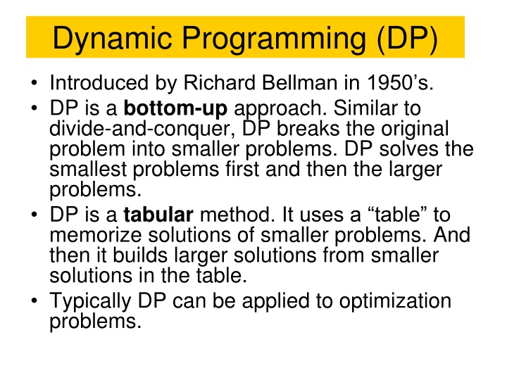
Dynamic programming (DP) is a bottom-up approach introduced by Richard Bellman in the 1950s. Similar to divide-and-conquer, DP breaks down complex problems into smaller subproblems, solving them methodically and storing solutions in a table for efficient computation. DP is widely used in optimization problems, with key elements including recurrence relations, tables for memorization, and algorithms for filling tables. An example of DP application is demonstrated through Fibonacci numbers and a canoe trip optimization problem.

  • Dynamic Programming
  • Bellman
  • Recurrence Relations
  • Optimization
  • Problem Solving

Uploaded on Sep 19, 2024 | 0 Views


Download Presentation

Please find below an Image/Link to download the presentation.

The content on the website is provided AS IS for your information and personal use only. It may not be sold, licensed, or shared on other websites without obtaining consent from the author. Download presentation by click this link. If you encounter any issues during the download, it is possible that the publisher has removed the file from their server.

E N D

Presentation Transcript


  1. Dynamic Programming (DP) Introduced by Richard Bellman in 1950 s. DP is a bottom-up approach. Similar to divide-and-conquer, DP breaks the original problem into smaller problems. DP solves the smallest problems first and then the larger problems. DP is a tabular method. It uses a table to memorize solutions of smaller problems. And then it builds larger solutions from smaller solutions in the table. Typically DP can be applied to optimization problems.

  2. Basic elements of a DP algorithm 1. A DP recurrence, i.e. a recursive relation between larger and smaller solutions. 2. A table for memorizing solutions. 3. An algorithm for filling the table.

  3. Fibonacci Numbers Recursive Fibonacci numbers: Int fib(int n) { if (n<2) return n; else return fib(n 1) + fib(n 2); } DP Fibonacci numbers: 1. fn = fn-1+fn-2 2. Int f[n+1]; /* f[i] contains fi */ 3. The algorithm. f[0] = 0; f[1] = 1; for (i=2; i<=n; ++i) f[i] = f[i-1] + f[i-2];

  4. A Canoe Trip Definition of the problem: There are n trading posts along a river. At any of the posts you can rent a canoe to be returned at any other post downstream. For each post i and each downstream post j, the cost of the rental from post I to post j is known. We want to know what is the best way to rent and return canoes from post 0 to post n-1.

  5. Defining subproblems (smaller problems) Define mc(i) as the minimum coast to travel from post 0 to post i. The DP recurrence mc(0) = 0 mc(i) = MIN { mc(j) + cost[j][i]} 0 j<i

  6. The table int mc[n]; // mc[i] contains min cost from post 0 to post i; The algorithm for filling the table mc[0] = 0; for (i=1; i<n; ++i) { mc[i] = cost[0][i]; prv[i] = 0; for (j=1; j<i; ++j) { temp = mc[j] + cost[j][i]; if (temp<mc[i]) { mc[i] = temp; prv[i] = j; } } } i = n-1; while (i>0) { printf("%d <-- ", i+1); i = prv[i]; } printf("%d\n", 0);

  7. Example 1 8 0 Cost 0 1 2 3 4 0 2 3 23 8 4 20 11 24 20 8 0 5 0 5 0 0 mc(i) = MIN { mc(j) + cost[j][i]} 0 j<i 0 0 1 8 0 2 19 1 3 16 1 4 mc prv 21 3 0 1 3 4

  8. Principle of optimality Principle of optimality: Suppose that in solving a problem, we have to make a sequence of decisions D1, D2, , Dn. If this sequence is optimal, then the last k decisions, 1 k n must be optimal. In solving an optimization problem, DP may be used only when the principle of optimality holds.

  9. Matrix Product Chain Review: Matrix Multiplication. C = A*B A is d e and B is e f f B 1 e = k = , [ i C ] , [ i A ] * [ , ] j k B k j j e 0 O(def ) time e A C d i i,j d f

  10. Matrix Product Chain Matrix product chain: Compute A=A0*A1* *An-1 Ai is di di+1 Problem: What is the best order? Example B is 3 100 C is 100 5 D is 5 5 (B*C)*D takes 1500 + 75 = 1575 multiplications B*(C*D) takes 1500 + 2500 = 4000 multiplications

  11. Defining subproblems Define Ni,j as the minimum number of multiplications needed for computing Ai*Ai+1* *Aj. The DP recurrence Ni,j = min {Ni,k +Nk+1,j+didk+1dj+1} i k<j

  12. The table answer N 1 2 1 0 2 j n 0 0 i 0 0 0 0 0 0 n 0 Ni,j = min {Ni,k +Nk+1,j+didk+1dj+1} i k<j

  13. The algorithm for (i=0; i<n; ++i) N[i][i] = 0; for (len=2; len<=n; ++len) { for (i = 0; i<n-len+1; ++i) { j = i + len 1; N[i][j] = ; for (k = i; k<j; ++k) { q = N[i][k] + N[k+1][j] + d[i]*d[k+1]*d[j+1]; if (q < N[i][j]) N[i][j] = q; } } }

  14. Example Ni,j = min {Ni,k +Nk+1,j+didk+1dj+1} i k<j 1 2 3 5 4 7 5 10 6 d 13 18 9 j N 1 2 3 4 5 1 2 3 4 5 810 k=1 1440 k=2 315 0 0 i 0 350 910 0 0

  15. Longest Common Subsequence Problem: Given 2 sequences, X = x1,...,xm and Y = y1,...,yn , find a common subsequence whose length is maximum. springtime ncaa tournament basketball printing north carolina krzyzewski Subsequence need not be consecutive, but must be in order.

  16. Nave Algorithm For every subsequence of X, check whether it s a subsequence of Y . Time: O(n2m). 2msubsequences of X to check. Each subsequence takes O(n)time to check: scan Y for first letter, for second, and so on.

  17. LCS properties Theorem Let Z = z1, . . . , zk be any LCS of X and Y . 1. If xm= yn then zk= xm= ynand Zk-1 is an LCS of Xm-1 and Yn-1. 2. If xm yn then either zk xmand Z is an LCS of Xm-1 and Y. 3. or zk ynand Z is an LCS of X and Yn-1. Notation: prefix Xi= x1,...,xi is the first i letters of X.

  18. Defining subproblems Define C(i, j) as length of LCS of Xi and Yj . We want C(m,n). The DP recurrence 0 if i=0 or j=0, C(i, j) = C(i-1, j-1)+1 if i,j>0 and xi=yj max { C(i-1, j), C(i, j-1)} if i,j>0 and xi yj

  19. The table C 0 1 0 0 0 0 0 0 0 0 0 0 0 1 0 j 0 n 0 0 0 0 0 0 0 i,j i answer m 0 if I=0 or j=0, C(I, j) = C(i-1, j-1)+1 if I,j>0 and xi=yj max { C(i-1, j), C(i, j-1) } if I,j>0 and xi=yj

  20. The algorithm for (i=1; i<=m; ++i) C[i][0] = 0; for (j=1; j<=n; ++j) C[j][0] = 0; for (i=1; i<=m; ++i) { for (j=1; j<=n; ++j) { if (xi == yj) { C[i][j ] = C[i 1][j 1] + 1; B[i, j ] = } else { if (C[i 1][j] C[i][j 1]) { C[I][j] = C[i 1][j]; B[i][j] = ; } else { C[i][j] = C[i][j 1]; B[i][j] = ; } } } } B[i][j] points to the entry whose subproblem we used in solving LCS of Xi and Yj. Time: O(mn)

  21. Finding LCS j 0 1 2 3 4 5 Yj B D i C A B Xi 0 0 0 0 0 0 0 A 0 0 0 0 1 1 1 B 2 0 1 1 1 1 2 C 3 0 1 1 2 2 2 B 4 0 1 1 2 3 2

  22. Finding LCS j 0 1 2 3 4 5 Yj B D i C A B Xi 0 0 0 0 0 0 0 A 0 0 0 0 1 1 1 B 2 0 1 1 1 1 2 C 3 0 1 1 2 2 2 3 B 4 0 1 1 2 2

  23. 0-1 Knapsack: an example Weight Value vi wi Objects 2 3 This is a knapsack Max weight: W = 20 3 4 4 5 5 8 9 10

  24. 0-1 Knapsack problem Given a knapsack with maximum capacity W, and a set of n objects. Each object i has a weight wi and a value vi(all wi , viand W are integer values). Problem: How to pack the knapsack to achieve maximum total value of packed objects?

  25. 0-1 Knapsack problem The problem, in other words, is to find: max vi subject to wi W i Ti T 1. The problem is called a 0-1 problem, because each object must be entirely accepted or rejected. 2. Just another version of this problem is the Fractional Knapsack Problem , where we can take fractions of objects.

  26. Brute-force approach Since there are n items, there are 2n possible combinations of items. We go through all combinations and find the one with the most total value and with total weight less or equal to W. Running time will be O(n2n).

  27. The DP approach Can we do better? Yes, with an algorithm based on dynamic programming. We need to identify the subproblems. Defining subproblems Define V(k,w) as the maximum total value if we only include objects 1 to k and if the capacity is w.

  28. The DP recurrence V(k-1, w) if wk >w V(k,w) = max{V(k-1, w), V(k-1, w-wk)+vk} The table V 0 1 0 1 2 w W K-1,w-wk K-1,w k k,w answer n

  29. The algorithm for filling the table for (w=0; w<=W; ++w) P[0][w] = 0; for (i=0; i<=n; ++i) { P[i][0] = 0; for (w=0; w<=W; ++w) if (wi <= W) /* object i can be included */ if (pi+P[i-1][w-wi]>P[i-1][w]) P[i][w] = pi + P[i-1][w- wi]; else P[i][w] = P[i-1][w]; else P[i][w] = P[i-1][w]; }

  30. Optimal Binary Search Trees Problem Given sequence K = k1< k2< < kn of n sorted keys, with a search probability pifor each key ki. Want to build a binary search tree (BST) with minimum expected search cost. Actual cost = # of items examined. For key ki, cost = depthT(ki)+1, where depthT(ki)= depth of kiin BST T .

  31. Expected Search Cost search [ cost in ] E T n = n = + ( depth ( ) ) 1 k p T i i 1 i n = i = i = + depth ( ) k p p T i i i 1 1 n = i = + 1 depth ( ) k p T i i Sum of probabilities is 1. 1

  32. Example 1 Consider 5 keys with these search probabilities: p1 = 0.25, p2 = 0.2, p3 = 0.05, p4 = 0.2, p5 = 0.3. k2 i depthT(ki) depthT(ki) pi 1 1 0.25 2 0 0 3 2 0.1 4 1 0.2 5 2 0.6 1.15 k1 k4 k3 k5 Therefore, E[search cost] = 2.15.

  33. Example 2 p1 = 0.25, p2 = 0.2, p3 = 0.05, p4 = 0.2, p5 = 0.3. k2 i depthT(ki)depthT(ki) pi 1 1 0.25 2 0 0 3 3 0.15 4 2 0.4 5 1 0.3 1.10 k1 k5 k4 Therefore, E[search cost] = 2.10. k3 This tree turns out to be optimal for this set of keys.

  34. Observations: Optimal BST may not have smallest height. Optimal BST may not have highest-probability key at root. Build by exhaustive checking? Construct each n-node BST. For each BST, compute expected search cost. But there are O(4n/n3/2)different BSTs with n nodes.

  35. Some properties of optimal BST One of the keys in ki, ,kj, say kr, where i r j, must be the root of an optimal subtree for these keys. Left subtree of krcontains ki,...,kr 1. Right subtree of krcontains kr+1, ...,kj. kr To find an optimal BST: Examine all candidate roots kr, for i r j Determine all optimal BSTs containing ki,...,kr 1 and containing kr+1,...,kj ki kr-1 kr+1 kj

  36. Defining subproblems Define e(i, j ) as expected search cost of optimal BST for ki,...,kj. The DP recurrence 0 if j=i-1, e(i, j) = min { e(i, r-1)+e(r+1, j)+w(i,j)} if i j i r j j = l = ( , ) w i j lp i

  37. The table answer e 1 2 0 0 1 j n 0 0 i 0 0 0 0 0 0 n+1 0 0 if j=i-1, e(i, j) = min { e(i, r-1)+e(r+1, j)+w(i,j)} if i j i r j

  38. The algorithm for (i=1; i<= n+1; ++i) e[i][i 1] = w[i][i 1] = 0; for (l=1; l<=n; ++I) { for (i=1; i<=n l+1; ++i) { j i + l 1; e[i][j] = ; w[i][j] = w[i][j 1] + pj; for (r=i; r<=j; ++r) { t = e[i][r 1] + e[r+1][j ] + w[i][j]; if (t<e[i][j]) { e[i][j ] = t; root[i][j ] = r; } } } }

  39. Home works 1. Complete the table on slide 14. 2. Given an array A of nonnegative integers such that A[i] represents the max number of steps that can be made forward from A[i]. Design a DP algorithm to determine how to use the minimum number of jumps to reach the end of the array A starting from A[0]. If A[i] is 0, then we cannot move through A[i]. Example: If A[] = {1, 3, 0, 8, 4, 2, 6, 7, 6, 8, 0}, the output is 3 (A[0] A[1] A[3] A[10]). A[0] is 1, so can only go to A[1]. A[1] is 3, so can make at most 3 steps i.e. to A[2] or A[3] or A[4].

Related


More Related Content

giItT1WQy@!-/#giItT1WQy@!-/#giItT1WQy@!-/#giItT1WQy@!-/#giItT1WQy@!-/#giItT1WQy@!-/#giItT1WQy@!-/#giItT1WQy@!-/#giItT1WQy@!-/#giItT1WQy@!-/#giItT1WQy@!-/#giItT1WQy@!-/#