Introduction to Deep Learning and Boltzmann Machines

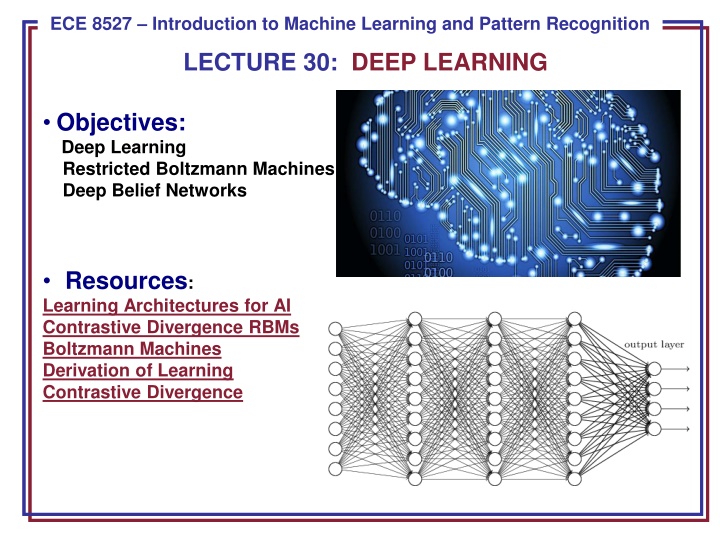
ECE 8443 Pattern Recognition ECE 8527 Introduction to Machine Learning and Pattern Recognition LECTURE 30: DEEP LEARNING Objectives: Deep Learning Restricted Boltzmann Machines Deep Belief Networks Resources: Learning Architectures for AI Contrastive Divergence RBMs Boltzmann Machines Derivation of Learning Contrastive Divergence

Deep Learning Deep learning is a branch of machine learning that has gained great popularity in the latest years The first deep network descriptions emerged in the late 60s and early 70s. Ivankhnenko (1971) published a paper that described a deep network with 8 layers trained by the Group Method of Data Handling algorithm In 1989 LeCun was able to apply the standard backpropagation algorithm to train a deep network to recognize handwritten Zip codes. This process was not very practical, since it took three days for training In 1998, a team led by Larry Heck achieved the first success for deep learning on speaker recognition. Nowadays, several speech recognition problems have been approached with a deep learning method called a Long Short Term Memory (LSTM), a recurrent neural network proposed by Schmidhuber in 1997 New training methodologies (greedy-layer-wise learning algorithm) and advances in hardware (GPUs) have contributed to the renewed interest on this topic. ECE 8527: Lecture 30, Slide 1

Vanishing Gradient and Backpropagation One of the reasons that made the training of deep neural networks a difficult task is related to the vanishing gradient, which results from gradient based training techniques and the backpropagation algorithm Considering a very simple deep network, with only one neuron per layer, a cost C and a sigmoid activation function: A small change in ?? sets off a series of cascading changes in the network ?? ?? ????+?? in the weighted input ??, which would be given by ?? ? ???? ??. Basically, a term ? (??) and ?? is picked up in every neuron ?? or ??= ? ?? ?? The chance in ??, then causes a change ??? The resulting change in cost (divided by ??), produced by the change ?? is given by: ?? ??? = ? ?? ?? ? ?? ?? ? ?? ?? ? ?? ?? ??? For a sigmoid, ? ? =? to a vanishing gradient <? ?, in this sense, the terms ??? ?? ?, contributing ECE 8527: Lecture 30, Slide 2

Boltzmann Machines (BM) The vanishing gradient results in very slow training for the front layers of the network One of the solutions to this issue was proposed by Hinton (2006). He proposed to use a Restricted Boltzmann Machine (RBM) to model each new layer of higher level features RBMs are energy based models, they associate a scalar energy to each configuration of the variables of interest RBM ?1 1 Energy based probabilistic models define a probability distribution as: ?2 2 ? ? =? ? ? where ? = ?? ? ? ? ?3 An energy-based model can be learnt by performing (stochastic) gradient descent on the empirical negative log-likelihood of the training data, where the log-likelihood and the loss function are: ? ? ??????? ?(??) 2 ?4 and ? ?,? = ?(?,?) ? ?,? = ECE 8527: Lecture 30, Slide 3

Boltzmann Machines (BM) RBMs consist of a visible layer v and a hidden layer h, so ? ? ?,? ? ? ? = ?? ?,? = ? Introducing the notation of free energy: ? ? = ??? ?? ?(?,?) we can write: ? ? =? ? ? with ? = ?? ? ? ? Then the data negative log-likelihood gradient has the following form: ?? ? ?? ????? ? =?? ? ? ? ?? ?? ? PositivePhase: increase probability of training data NegativePhase: Decrease probability of samples generated by model Usually, samples belonging to N are used to estimate the gradient. The elements ? of N are sampled according to P: ?? ? ?? ????? ? =?? ? ? ? ? |?| ??? ?? ?? ECE 8527: Lecture 30, Slide 4

Restricted Boltzmann Machines (RBM) RBMs have energy functions that are linear in their free parameters. Some of the variables are never observed (hidden) and restrict BMs to those without interconnections in the same layer The energy function for an RBM with weights W is ? ?,? = ? ? ? ? ? ?? or ? ? = ? ? ???? ???????+??? Where b and c are offsets of the visible and hidden layers Given that visible and hidden units are conditionally independent given one another: ? ? ? = ?? ??? and ? ? ? = ??(??|?) If using binary units, the free energy and the probabilistic version of the activation function are given by: ? ? = ? ? ???(? + ???+???) ? ? ??= ? ? = ? ??+ ??? ? ??= ? ? = ?(??+ ? ??) ECE 8527: Lecture 30, Slide 5

Restricted Boltzmann Machines (RBM) Considering the previous information, the update equations are theoretically given by: ???? ? ? ???? ? ? ?? ??+ ?? = ??? ??? ?? ?? ???? ? ? ? ?? ?? = ??? ??? ??? ???? ? ? (?) = ??? ??? ?? ??? In practice, the log-likelihood gradients are commonly approximated by algorithms such as Contrastive Divergence (CD-k), which does the following: Since we want ? ? ??????? a Markov Chain is initialized with a training example that is close to p (so chain is close to convergence) CD selects samples after only k steps of Gibbs sampling (does not wait for convergence) ECE 8527: Lecture 30, Slide 6

RBM Training Summary 1. Forward Pass: Inputs are combined with an individual weights and a bias. Some hidden nodes are activated. 2. Backward Pass: Activations are combined with an individual weight and a bias. Results are passed to the visible layer. 3. Divergence calculation: Input ? and samples ? are compared in visible layer. Parameters are updated and steps are repeated ?? ? ?1 ?? ????? ? 2 ?? ?2 1 ?? ? ?? 1 3 2 ?1 ?2 ?? Input being passed to first hidden node 2 ?2 3 1 ?1 3 Activations are passed to visible layer for reconstruction 2 ?2 ?????? ?,?,? 3 ?? activates in this example ECE 8527: Lecture 30, Slide 7

Deep Belief Networks (DBN) These networks can be seen as a stack of RBMs. The hidden layer of one RBM is the Visible layer of the one above it A pre-training step is done by training the layers one RBM at a time. The output for one set is used as the input for the next one ???1???2 ???3???4 In this sense, each RBM layer learns the entire input. The DBN fine tunes the entire input in succession as the model improves. This is called unsupervised, layer-wise, greedy pre-training ECE 8527: Lecture 30, Slide 8

Supervised Fine-Tuning of DBNs After unsupervised pre-training, the network can be further optimized by gradient descent with respect to a supervised training criterion. As a small set of labeled samples is introduced, the parameters are slightly updated to improve the network s perception of the patterns Labels This training process can be accomplished in a reasonable amount of time (depending on the depth and other parameters of the DBN) in a GPU Given that DBN attempt to sequentially learn the entire input and then reconstruct it in a backward pass, they are commonly used to learn features for the data. ECE 8527: Lecture 30, Slide 9

Example: Movie Recommendations In this example, a simple RBM will be constructed and utilized for movie recommendations In 2007, Hinton proposed the utilization of RBMs in order to produce more accurate movie recommendations with Netflix data Essentially, the input data is comprised of the movies that users liked. The output is a set of weights that activate (or not) the hidden units that, in this case will represent movie genre. As it was shown in the RBM training section, the input will be passed to the hidden layer, where the activation energy is calculated and the weights and biases are updated The input is then attempted to be reconstructed in a similar manner and the hidden units are updated accordingly In this example the visible units will represent a movie and the input will be 1 if the user liked it, and 0 if the user did not like it For a new user, the activation (or not activation) of the hidden units, indicates whether or not the use should be recommended to a set of movies Note that this is a simple example to illustrate one application of RBMs. ECE 8527: Lecture 30, Slide 10

Example: Movie Recommendations The RBM used in this example is constructed to have 6 visible units and 2 hidden units ??:????? ?????? ??:?????? ??:???? ?? ??? ????? ? Hidden Layer ??:????????? ??:??????? ??:??????? Visible Layer ?? ?? ?? ?? ?? ?? Input for Training User#: ?? ?? ?? ?? ?? ?? User1: [1 1 1 0 0 0] User2: [1 0 1 0 0 0] User3: [1 1 1 0 0 0] User4: [0 0 1 1 1 0] User5: [0 0 1 1 0 1] User6: [0 0 1 1 1 0] In this case, the hidden units will learn two latent variables underlying preferences. the movie For example: It could learn to identify the Sci- Fi/Fantasy movies from the Oscar winning movies 1: User liked the movie 0: User did not like the movie ECE 8527: Lecture 30, Slide 11

Example: Movie Recommendations Running the code for the specified RBM and the provided examples produces the following weights: The probability of activation is the sigmoid of the activation energy, negative values will correspond to low probability of activation. It can be seen that the first hidden layer activates for Sci-Fi/Fantasy movies, while the second hidden layer corresponds to Oscar Winners. When entering the information of a new user that likes Titanic and Gladiator, we get this result: In this sense, the system is more likely to recommend Oscar Winning Movies to the new user. ECE 8527: Lecture 30, Slide 12

Summary Deep learning has gained popularity in the latest years due to hardware advances (GPUs, etc.) and new training methodologies, which helped overcome the issue of the vanishing gradient RBMs are shallow 2 layer networks (visible and hidden) that can find patterns in data by reconstructing the input in an unsupervised manner. RBM training can be accomplished through algorithms such as Contrastive Divergence (CD) To learn more: https://deeplearning4j.org/restrictedboltzmannmachine ECE 8527: Lecture 30, Slide 13