Introduction to Data Analysis in Geophysics with Seismic Analysis Code - SAC Lab 2.1

Explore the world of geophysics data analysis using the SAC Lab 2.1 code. Learn about seismic analysis, Fourier transform analysis, spectral analysis, color tracing, integration, differentiation, and more. The SAC online documentation provides valuable resources for users to delve deeper into this fascinating field.

• Geophysics
• Seismic Analysis
• Data Analysis
• Fourier Transform
• Spectral Analysis

lyeat Follow

Uploaded on Sep 07, 2024 | 0 Views

Download Presentation

Please find below an Image/Link to download the presentation.

The content on the website is provided AS IS for your information and personal use only. It may not be sold, licensed, or shared on other websites without obtaining consent from the author. Download presentation by click this link. If you encounter any issues during the download, it is possible that the publisher has removed the file from their server.

Presentation Transcript

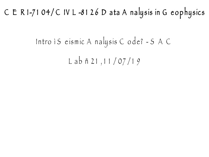
1. C E R I C E R I- -7 1 04/ C IV L 7 1 04/ C IV L - -8 1 2 6 D ata A nalysis in G eophysics 8 1 2 6 D ata A nalysis in G eophysics Intro S eismic A nalysis C ode - S A C L ab 2 1 , 1 1 / 07 / 1 9

2. S A C online documentation S A C online documentation https:/ / ds.iris.edu/ files/ sac-manual/ manual.html

3. C an color traces (this is an addition since the T E K 401 X days when it was green or nothing). SAC> color on increment on SAC> p2 Sac> p2 rel

4. S pectral A nalysis M odule (SAM): S pectral/ F ourier T ransform analysis. Y ou can do a discrete F ourier transform fft and an inverse F ourier transform ifft Y ou can also compute the amplitude and unwrapped phase of a signal ( unwrap ). T his is an implementation of the algorithm due to T ribolet.

5. T he fft and unwrap commands produce spectral data in memory. Y ou can plot this spectral data plotsp

6. Y ou can also perform - integration with divomega and - differentiation with mulomega directly in the frequency domain.

7. sac> funcgen seismogram sac> fft sac> plotsp P lots amplitude T hen the phase after a <C R >

8. U N W R A P SAC> cut 3000 5000 SAC> read *india*bhz* SAC> qdp off SAC> p SAC> rtrend SAC> UNWRAP FILL OFF INTTHR 10 PVTHR 5 DC level after DFT is 53.572 SAC> psp P lots amplitude T hen the unwrapped phase after a <C R >

9. Y ou can write it to disk as writesp and read in back in again readsp Y ou have to know the data/ file is spectral data. S A C will not figure it out.

10. S pectral A nalysis M odule (SAM): S pectral/ F ourier T ransform analysis. Y ou can also correlate correlate and convolve convolve H as lots of options see online man page https://ds.iris.edu/files/sac-manual/commands/correlate.html

11. C onvolution ex. S tart with D W W S S N impulse response IR what the seismometer records if you apply an impulse.

12. C onvolution ex. If we zoom in we can see that the IR starts at 2 00 seconds and is done by 2 7 0 seconds.

13. C onvolution ex. N ow make a series of impulses and save them. fg impstrin 300 500 600 630 750 760 770 780 n 1024

14. C onvolution ex. R ead in file with IR & file with series of impulses and convolve them. R esult is sum of series of weighted, shifted IR s.

15. C onvolution ex. Z oom into the third signal.

16. C onvolution ex. Z oom into the fourth signal. SAC> fg impstrin 200 n 1024 SAC> transfer to DWWSSN SAC> w sac ir_200_l1024.sac SAC> fg impstrin 300 500 600 630 750 760 770 780 n 1024 SAC> w sac imps.sac SAC> read ir_200_l1024.sac imps.sac SAC> convolve look at it, then zoom in SAC> xlim 770 910 look at it, then zoom again SAC> xlim 940 1060 SAC> w sac ximps.sac 8imps.sac

17. W e can use the transfer command to remove the IR and recover the input to the seismometer. SAC> transfer from DWWSSN to none

18. C orrelation ex. C orrelation looks for one signal in another. L ook for IR in the seismograms . It returns a set of weighted, shifted peaked functions.

19. S ignal C orrection M odule T hese commands let you perform certain signal correction operations. - rmean: removes the mean from data. - rtrend: removes linear trend (and mean) from data.

20. - rglitches: removes glitches and timing marks. - taper: applies a symmetric taper to each end of the data and SMOOTH applies an arithmetic smoothing algorithm. - linefit: computes the best straight line fit to the data in memory and writes the results to header blackboard variables. - reverse: reverses the order of data points.

21. Integration to change from acceleration to velocity, and velocity to displacement. SAC> r ccm_india_.bhz SAC> qdp off SAC> plot

22. Integrate it (original data was vel, integrate to disp). SAC> int SAC> p O O P S !

23. W hat is the problem? (do you agree that there is a problem?!)

24. Integral of constant is a straight sloping line. T he seismic data has a (small) D C offset (a constant). S o remove the mean.

25. T ry again. SAC> r SAC> rmean SAC> int SAC> p O O P S again!

26. Is this an improvement? A re we getting any better? W hat s the problem now?

27. Integral of linear fn (line) is a quadratic fn (parabola). S o data has a linear trend - remove trend (line) from data (y=mx+b) (this will also remove the mean through the intercept b).

28. R emove trend (line) with rtrend, this removes y= mx+ b both the line and the D C offset SAC> r SAC> rtrend Slope and standard deviation are: -0.038705 0.0037565 Intercept and standard deviation are: -2365.1 15.788 Data standard deviation is: 3010.9 Data correlation coefficient is: 0.026988 SAC> int SAC> p

29. R emoving the line will also remove the mean if it is not zero. S o don t really need to do the rmean first.

30. T here is still some drift , but this seismogram might be useful for displacement analysis. SAC> r SAC> rtrend Slope and standard deviation are: -0.038705 0.0037565 Intercept and standard deviation are: -2365.1 15.788 Data standard deviation is: 3010.9 Data correlation coefficient is: 0.026988 SAC> int SAC> r more SAC> p1 S A C > r more S A C > p1 displacement velocity

31. B ig problems with "baseline" drift when trying to integrate acceleration up to displacement to when trying to obtain/ estimate co-seismic static displacement. B oore, 2 001

32. D ifferentiation - default is 2 point difference y=(x1-x0)/delta. sac> funcgen impulse delta 0.01 npts 100 sac> dif sac> p

33. D ifferentiate velocity to acceleration. SAC> r SAC> dif SAC> p

34. M ore on correlation SAC> r *india*z SAC> correlate SAC> p W hat s wrong here?

35. M ore on correlation SAC> fg boxcar SAC> p SAC> correlate SAC> p B oxcar S ignal C orrelation

36. M ore on correlation SAC> r *india*z SAC> rtrend SAC> correlate SAC> p F ix by removing mean with rmean, or better yet, remove trend (gets mean and linear) with rtrend.

37. M ore on correlation SAC> r US.WRAK..BHZ.M.2011.070.055503.SAC *SCIA*Z* SAC> p1

38. M ore on correlation SAC> rtrend SAC> correlate SAC> p1

39. B inary O perations M odule T hese commands perform operations on pairs of data files. - merge: merges (concatenates) a set of files to the data in memory.

40. B inary O perations M odule - addf: A dds a set of data files to data in memory. READ FILE1 FILE2 ADDF FILE3 FILE4 READ FILE1 FILE2 FILE3 ADDF FILE4 - subf: subtracts a set of data files from the ones in memory.

41. - mulf: multiplies the data in memory by a set of data files. - divf: divides the data in memory by a set of files. - binoperr: controls errors that can occur during these binary operations. C an use to override the requirement for the same number of points and/ or the same sampling interval.

42. sac> funcgen impulse delta 0.01 npts 100 sac> w impulse1.sac sac> div 2 sac> w impulse2.sac sac> r impulse1.sac sac> addf impulse2.sac N otice you have to write intermediate stuff out to disk.

43. W indowing SAC> funcgen sine 10 90 delta 0.01 npts 100 SAC> TAPER TYPE HANNING WIDTH 0.5 SAC> w sac taper0.5.sac SAC> funcgen sine 10 90 delta 0.01 npts 100 SAC> r more ./taper0.5.sac SAC> color on increment on SAC> p2

44. M ore - stretch -upsamples data, including an optional interpolating F IR filter. - decimate -downsamples data, including an optional anti-aliasing F IR filter (this is what qdp does without the filter). - Interpolate - interpolate evenly or unevenly spaced data to a new sampling interval using the interpolate command.

45. M ore - quantize -converts continuous data into its quantized equivalent. - rotate -pairs of data components through a specified angle. (we have already seen this one) - rq - removes the seismic Q factor from spectral data.