Gravity and Magnetic Models in Geophysics

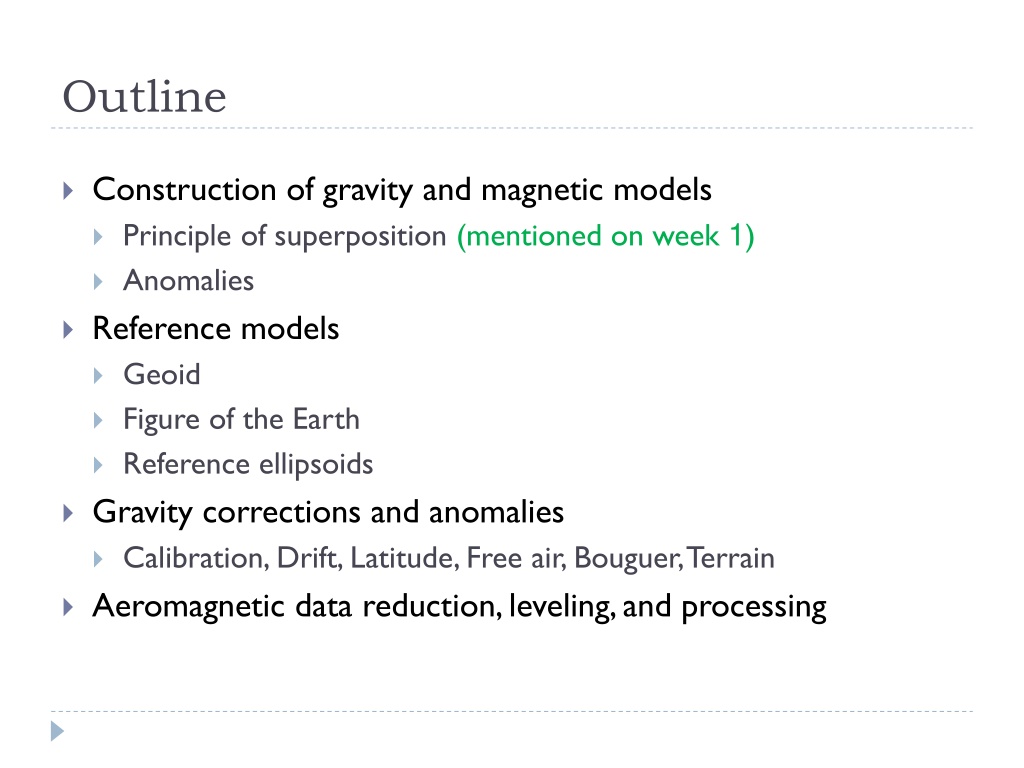
Construction of gravity and magnetic models involves principles of superposition to isolate anomalies, reference ellipsoids, geoid, and various corrections like drift, latitude, free air, Bouguer, and terrain corrections. Gravity anomalies are determined by subtracting multiple factors from observed gravity measurements. The geoid represents the actual equipotential surface at mean sea level, while the reference ellipsoid is a uniform Earth surface determined with GPS and satellite data. Hydrostatic rotating Earth models and gravity flattening concepts are also discussed.

• Geophysics
• Gravity models
• Magnetic models
• Anomalies
• Geoid

malan Follow

Uploaded on Sep 10, 2024 | 0 Views

Download Presentation

Please find below an Image/Link to download the presentation.

The content on the website is provided AS IS for your information and personal use only. It may not be sold, licensed, or shared on other websites without obtaining consent from the author. Download presentation by click this link. If you encounter any issues during the download, it is possible that the publisher has removed the file from their server.

Presentation Transcript

1. Outline Construction of gravity and magnetic models Principle of superposition (mentioned on week 1) Anomalies Reference models Geoid Figure of the Earth Reference ellipsoids Gravity corrections and anomalies Calibration, Drift, Latitude, Free air, Bouguer, Terrain Aeromagnetic data reduction, leveling, and processing

2. Gravity anomalies The isolation of anomalies (related to unknown local structure) is achieved through a series of corrections to the observed gravity for the predictable regional effects According to Blakely (page 137), it is best to view the corrections as superposition of contributions of various factors to the observed gravity (next slide)

3. Gravity anomalies Observed gravity = attraction of the reference ellipsoid (figure of the Earth) + effect of the atmosphere (for some ellipsoids) + effect of the elevation above sea level (free air) + effect if the average mass above sea level (Bouguer and terrain) + time-dependent variations (drift and tidal) + effect of moving platform (E tv s) + effect of masses that would support topographic loads (isostatic) + effect of crust and upper mantle density ( geology ) If we model and subtract these terms from the data then the remainder is the anomaly (for example, free air or Bouguer gravity)

4. Geoid and Reference Ellipsoid Geoid is the actual equipotential surface at (regional) mean sea level Reference ellipsoid is the equipotential surface in a uniform Earth Much more precisely known from GPS and satellite gravity data Recent recommendations are to reference all corrections to the reference ellipsoids and not to the geoid

5. Hydrostatic rotating Earth The surface of static fluid is at constant potential : 1 , 2 Gravity potential ( ) ( ) ( ) = = 2 2 2 sin U r g r R r const g r R polar Centrifugal potential 1 2 ( ) 2 2 2 sin g r polar r R Therefore: 2 2 3 R g R ( ) ( ) + 2 = = polar1 r sin r f f where: 2 2 GM Conventionally, the equatorial radius is used for referencing: ( ) ( 1 e r r ) 2 cos f

6. Gravity flattening Because of rotation, gravity decreases with colatitude : ( ) , U r g g r ( ) ( ) = = + 2 2 2 sin 1 cos r g e 2 R = = 2 f where g so that the gravity at the pole equals ( ) + 1 g g p e Parameter is called gravity flattening : g g = p e g e

7. Reference Ellipsoids International Gravity Formula Established in 1930; IGF30 Updated: IGF67 World Geodetic System (last revision 1984; WGS84) Established by U.S. Dept of Defense Used by GPS So the gravity field is measured above the atmosphere The difference from IGF30 can be ~100 m A number of other older ellipsoids used in cartography Also note the International Geomagnetic Reference Field: IGRF-11

8. Gravity flattening and the shape of the Earth Exercise: from the expressions for the Earth s figure and gravity flattening, show that the radius at colatitude can be estimated from measured gravity as: ( ) g g 5 2 ( ) = + 2 1 cos r r m e e

9. Multi-year drift of our gravity meter During field schools, the G267 gravimeter usually drifts by 0.1-0.2 mGal/day

10. Bullard B correction Necessary at high elevations (airborne gravity) Added to Bouguer slab gravity (subtracted from Bouguer-corrected gravity) to account for the sphericity of the Earth Bullard B correction (mGal) Elevation above reference ellipsoid, h (m) + 3 7 2 14 3mGal (with i 1.464 10 3.533 10 4.5 10 n meters) B B h h h h

11. Instrument Drift correction During the measurement, the instrument is used at sites with different gravity gs and also experiences a time-dependent drift d(tobs) Therefore, the value measured at time tobs at station s is: ( ) obs s s u t g = ( ) + d t (*) obs For d(t), we would usually use some simple dependence; for example, a polynomial function: ( ) 0 k = n = k d t a t d 0 k where d0 is selected to ensure zero mean: <d(t)> = 0, that is: ( ) n ( ) = k k d t a t t k = 0 k

12. Instrument Drift correction (cont.) Equation (*) is a system of linear equations with respect to all gs and ak: = Lm u where m is a vector of all unknowns: g g 1 2 ... a a m 0 1 ...

13. Instrument Drift correction (cont.) u is a vector of all observed values: ( ) ( ) 2 ... t t u t u t 1 1 1 u ( ) ( ... u n m ) u + 1 n m

14. Instrument Drift correction (cont.) and matrix L looks like this: ) ( ) ( ) ) ( ( 2 1 2 1 0 ... t t t t First columns correspond to gravity stations 1 2 2 2 1 0 ... t t t t 2 ... ... ... ... ... Last columns correspond to n drift correction terms ) ( ) ( ) ( ) ) ) ( ( ( 2 3 2 L 0 1 ... t t t t 3 2 4 2 0 1 ... t t t t 4 Rows correspond to recording times 2 5 2 0 1 ... t t t t 5 ... ... ... ... ...

15. Instrument Drift correction (finish) Then, the Least Squares solution of this matrix equation is achieved simply by: ( ) 1 = T T m L L L u In Matlab, this can be written as: = m u L \ Vector m contains all drift terms and all drift-corrected gravity values at all stations considered