Graph Embeddings in Online Social Networks and Media
Explore the concept of graph embeddings in online social networks for link prediction, classification, and feature engineering. Learn how graph embeddings map nodes to vectors and why they are essential in the machine learning lifecycle, with applications in tasks like link prediction and community detection.

Download Presentation

Please find below an Image/Link to download the presentation.
The content on the website is provided AS IS for your information and personal use only. It may not be sold, licensed, or shared on other websites without obtaining consent from the author. If you encounter any issues during the download, it is possible that the publisher has removed the file from their server.
You are allowed to download the files provided on this website for personal or commercial use, subject to the condition that they are used lawfully. All files are the property of their respective owners.
The content on the website is provided AS IS for your information and personal use only. It may not be sold, licensed, or shared on other websites without obtaining consent from the author.
E N D
Presentation Transcript
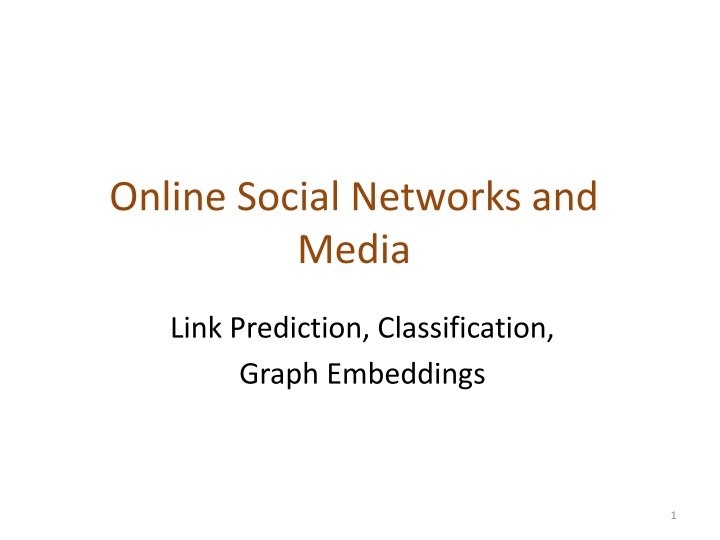
Online Social Networks and Media Link Prediction, Classification, Graph Embeddings 1
Graph embeddings: what are they? vec node u ?:? ? ? Feature representation, embedding Map nodes to d-dimensional vectors so that: similar nodes in the graph have embeddings that are close together. 2
Example Zachary s Karate Club Network: Input Output Image from: Perozzi et al.. DeepWalk: Online Learning of Social Representations. KDD 2014. 3
Graph embeddings: why? Machine learning lifecycle Raw Data Structured Data Learning Algorithm Model Feature Engineering Downstream prediction task degree, PageRank, motifs, degrees of neighbors, Pagerank of neighbors, etc 4
Graph embeddings: why? Machine learning lifecycle Raw Data Structured Data Learning Algorithm Model Feature Engineering Downstream prediction task degree, PageRank, motifs, degree of neighbors, Pagerank of neighbors, etc Automatically learn the features (embeddings) 5
Machine Learning tasks in networks Link prediction and link recommendations Node labeling Community detection (we have already seen an approach) Network similarity 6
Motivation Recommending new friends in online social networks, suggesting interactions or collaborations, predicting hidden connections (e.g., terrorist), In social networks: Increases user engagement Controls the growth of the network 8
Outline Estimating a score for each edge (seminal work of Liben- Nowell&Kleinberg) Classification approach The who to follow service at Twitter (one more application of link analysis) 9
Problem Definition Link prediction problem: Given the links in a social network at time t (Gold), predict the edges that will be added to the network during the time interval from time t to a given future time t (Gnew). Based solely on the topology of the network (social proximity) (the more general problem also considers attributes of the nodes and links) Different from the problem of inferring missing (hidden) links (there is a temporal aspect) To save experimental effort in the laboratory or in the field 10
Approach Assign a connection weight score(x, y) to each pair of nodes <x, y> based on the input graph Produce a ranked list of edges in decreasing order of score Recommend the ones with the highest score Note We can consider all links incident to a specific node x, and recommend to x the top ones If we focus to a specific x, the score can be seen as a centrality measure for x 11
How to define the score How to assign the score(x, y) between two nodes x and y? Some form of similarity or node proximity Two general methods Neighbors Paths 12
Neighborhood-based metrics The larger the overlap of the neighbors of two nodes, the more likely the nodes to be linked in the future Common neighbors: A adjacency matrix ??,? paths of length 2 2: number of different ????? ?,? = ? ? ? ? Jaccard coefficient: The probability that both x and y have a feature from a randomly selected feature that either x or y has |? ? ? ? | |? ? ? ? | ????? ?,? = 13
Neighborhood-based metrics Adamic Adar: 1 ????? ?,? = log(|? ? |) ? |? ? ? ? | Weighted version: common neighbors which themselves have few neighbors get larger weights (larger weights to rare features) Neighbors who are linked with 2 nodes are assigned weight = 1/log(2) Neighbors who are linked with 5 nodes are assigned weight = 1/log(5) Note: |N(x)| = degree of x, inverse logarithmic centrality 14
Neighborhood-based metrics Preferential attachment: ????? ?,? = ? ? |? ? | Nodes like to form ties with popular nodes E.g., empirical evidence suggest that co-authorship is correlated with the product of the neighborhood sizes Fall-back strategy: recommending popular users Depends on the degrees of the nodes not on their neighbors per se 15
Path-based methods score(x, y) = (negated) length of shortest path between x and y Not just the shortest, but all paths between two nodes Katz measure: ? ??|??? <?,?> | ?=1 Sum over all paths of length l 0 < < 1 parameter of the predictor, exponentially damped to count short paths more heavily 16
Path-based methods Katz measure: ??|??? <?,?> ? | = ? ??+ ?2??? 2+ ?3??? 3+ ?=1 ( ) 1 0 < < 1 Weighted version Small much like common neighbors small: degree, maximal: eigenvalue 17
Path-based methods Based on random walks that starts at x Hitting Time Hx,yfrom x to y: the expected number of steps it takes for the random walk starting at x to reach y. score(x, y) = Hx,y Commute Time Cx,yfrom x to y: the expected number of steps to travel from x to y and from y to x score(x, y) = (Hx,y+ Hy,x) Not symmetric, can be shown 18
Path-based methods Example: hit time h1,nin a line 1 i-1 i i+1 n Stationary-normed versions: to counteract the fact that Hx,yis rather small when y is a node with a large stationary probability regardless of x score(x, y) = Hx,y y score(x, y) = (Hx,y y+ Hy,x x) Personalized (or, Rooted) PageRank: with probability (1 a) moves to a random neighbor and with probability a returns to x score(x, y) = stationary probability of y in a personalized PageRank 19
SimRank Two objects are similar, if they are related to similar objects x and y are similar, if they are related to objects w and z respectively and w and z are themselves similar ? (?) ? ?(?)??????????(?,?) ? ? |? ? | ??????????(?,?) = ? Base case: similarity(x, x) = 1 score(x, y) = similarity(x, y) 20
SimRank Introduced for directed graphs: two objects are similar if referenced by similar objects ? ? ? ? ? ? ?,? = ? ? | ? ? | ?(?? , ?(?)) ?=1 ?=1 Average similarity between in-neighbors of a and in-neighbors of b I(x): in-neighbors of x, C: constant between 0 and 1, decay s(a, b) = 1, if a =b Iterative computation s0(x, y) = 1 if x = y and 0 otherwise sk+1based on the skvalues of its (in-neighbors) computed at iteration k 21
SimRank: the Pair Graph Pair graph G2 A node for each pair of nodes An edge (x, y) (a, b), if x a and y b a value per node: similarity of the corresponding pairs Computation starts at singleton nodes (score = 1) Scores flow from a node to its neighbors C gives the rate of decay as similarity flows across edges (C = 0.8 in the example) Symmetric pairs: (a, b) node same as (b, a) node (with the union of associated edges) Omit singleton that do not contribute to score (no {ProfA, ProfA} node) and nodes with 0 score {ProfA, StudentA}) Self-loops and cycles reinforce similarity Prune: by considering only nodes within a radius
SimRank and random walks Expected Meeting Distance (EMD) m (a, b) between a and b: the expected number of steps required before two random surfers, one starting at a and the other starting at b, would meet if they walked the graph randomly at lock-step m(u, v) = m(u,w) = , m(v, w) = 1 v and w are much more similar than u is to v or w. = 3, a lower similarity than between v and w but higher than between u and v (or u and w). = 23
SimRank and random walks Let us consider G2 A node (a, b) as a state of the tour in G: if a moves to c, b moves to d in G, then (a, b) moves to (c, d) in G2 A tour in G2of length n represents a pair of tours in G where each has length n What are the states in G2that correspond to meeting points in G? What is the meeting point of a and b? m(a, b)? 24
SimRank and random walks What are the states in G2that correspond to meeting points in G? Singleton nodes (common neighbors) The EMD m(a, b) is just the expected distance - hitting time in G2 between (a, b) and any singleton node The sum is taken over all walks that start from (a, b) and end at a singleton node This roughly corresponds to the SimRank of (a, b): when two surfers one from a and one from b that randomly walk the graph would meet 25
SimRank for bipartite graphs People are similar if they purchase similar items. Items are similar if they are purchased by similar people Useful for recommendations in general 26
SimRank IJCAI Philip S. Yu Q: What is most related conference to ICDM? KDD Ning Zhong ICDM R. Ramakrishnan SDM M. Jordan AAAI NIPS Author Conference 28
SimRank PKDD SDM PAKDD 0.008 0.007 0.009 KDD ICML 0.005 0.011 ICDM 0.005 0.004 CIKM ICDE 0.005 0.004 0.004 ECML SIGMOD DMKD 29
Evaluation of link recommendations Output a list Lpof pairs in V V Eoldranked by score predicted new links in decreasing order of confidence Precision at recall How many of the top-n predictions are correct where n = |Enew| Improvement over baseline Baseline: random predictor Possible correct Probability that a random prediction is correct: |V| Possible predictions 30
Can we combine the various scores? How? Classification (supervised learning) 31
Using Supervised Learning Given a collection of records (training set ) Each record contains a set of attributes (features) + the class attribute. Find a model for the class attribute as a function of the values of other attributes. Goal: previously unseen records should be assigned a class as accurately as possible. A test set is used to determine the accuracy of the model. Usually, the given data set is divided into training and test sets, with training set used to build the model and test set used to validate it. 33
Illustrating the Classification Task Learning algorithm Attrib1 Attrib2 Attrib3 Class Tid No 1 Yes Large 125K No 2 No Medium 100K No 3 No Small 70K Induction No 4 Yes Medium 120K Yes 5 No Large 95K No 6 No Medium 60K Learn Model No 7 Yes Large 220K Yes 8 No Small 85K No 9 No Medium 75K Yes 10 No Small 90K Model 10 Training Set Apply Model Attrib1 Attrib2 Attrib3 Class Tid ? 11 No Small 55K ? 12 Yes Medium 80K Deduction ? 13 Yes Large 110K ? 14 No Small 95K ? 15 No Large 67K 10 Test Set 34
Classification Techniques Decision Tree based methods Rule-based methods Memory based reasoning Neural networks (more soon) Na ve Bayes and Bayesian Belief networks Support vector machines Logistic regression 35
Example of a Decision Tree Splitting Attributes Tid Refund Marital Status Taxable Income Cheat No 1 Yes Single 125K Refund No 2 No Married 100K Yes No No 3 No Single 70K No 4 Yes Married 120K NO MarSt Yes 5 No Divorced 95K Married Single, Divorced No 6 No Married 60K TaxInc NO No 7 Yes Divorced 220K < 80K > 80K Yes 8 No Single 85K No 9 No Married 75K YES NO Yes 10 No Single 90K 10 Model: Decision Tree Training Data 36
Classification for Link Prediction Input Features describing the two nodes Output Prediction 37
Metrics for Performance Evaluation Confusion Matrix: PREDICTED CLASS Class=Yes Class=No ACTUAL CLASS Class=Yes TP FN Class=No FP TN + TP TN = Accuracy + + + TP TN FP FN 38
ROC Curve TPR (sensitivity)=TP/(TP+FN) (percentage of positive classified as positive) FPR = FP/(TN+FP) (percentage of negative classified as positive) (0,0): declare everything to be negative class (1,1): declare everything to be positive class (0,1): ideal Diagonal line: Random guessing Below diagonal line: prediction is opposite of the true class AUC: area under the ROC 39
Classification for Link Prediction: features For each edge (i, j) PropFlow: corresponds to the probability that a restricted random walk starting at x ends at y in l steps or fewer using link weights as transition probabilities (stops in l steps or if revisits a node) 40
How to construct the training set When to extract features and when to determine class? Two time instances x and y From t0to x construct graph and extract features (Gold) From x + 1 to yexamine if a link appears (determine class value) What are good values Large x better topological features (as the network reaches saturation) Large ylarger number of positives (size of positive class) Should also match the real-world prediction interval 41
How to construct the training set Unsupervised (single feature) 42
Datasets 712 million cellular phone calls weighted, directed networks, weights correspond to the number of calls use the first 5 weeks of data (5.5M nodes, 19.7M links) for extracting features and the 6th week (4.4M nodes, 8.5M links) for obtaining ground truth. 19,464 condensed matter physics collaborations from 1995 to 2000. weighted, undirected networks, weights correspond to the number of collaborations two authors share. use the years 1995 to 1999 (13.9K nodes, 80.6K links) for extracting features and the year 2000 (8.5K nodes, 41.0K links) for obtaining ground truth. The assortativity coefficient is the Pearson correlation coefficient of degree between pairs of linked nodes. Positive values indicate a correlation between nodes of similar degree, while negative values indicate relationships between nodes of different degree. 43
Using Supervised Learning: why? A different prediction model for each distance Predictors that work well in one network not in another Should increase with the score (not in phone) Preferential attachment increase with distance (when other may fail) 44
Using Supervised Learning: why? Even training on a single feature may outperform ranking (if no clear bound on score) Dependencies between features use an ensemble of features 45
Imbalance Sparse networks: |E| = k |V| for constant k << |V| The class imbalance ratio for link prediction in a sparse network is (|V|/1) when at most |V| nodes are added Missing links is |V|2 Positives V n-neighborhood exactly n hops way Treat each neighborhood as a separate problem 46
Results Ensemble of classifiers: Random Forest Random forest: Ensemble classifier constructs a multitude of decision trees at training time output the class that is the mode (most frequent) of the classes (classification) or mean prediction (regression) of the individual trees. 47
Results 48
Results Mechanism by which links arise different both across networks and geodesic distances. Local vs Global (preferential attachment) Better in condmat network, Improves with distance HPLP achieves performance levels as much as 30% higher than the best unsupervised methods 49
Salsa 50