GIS and Remote Sensing for Overlay Analysis Training Program

This training program focuses on GIS and remote sensing techniques for overlay analysis, covering topics such as data processing, suitability mapping, sensitivity analysis, and introduction to Python. The program includes practical sessions on QGIS, lithology, land use, recharge, TWI, and more. Participants will learn about data acquisition, pre-processing, overlaying, sensitivity analysis, and advanced geo-algorithms.

Download Presentation

Please find below an Image/Link to download the presentation.
The content on the website is provided AS IS for your information and personal use only. It may not be sold, licensed, or shared on other websites without obtaining consent from the author.If you encounter any issues during the download, it is possible that the publisher has removed the file from their server.
You are allowed to download the files provided on this website for personal or commercial use, subject to the condition that they are used lawfully. All files are the property of their respective owners.
The content on the website is provided AS IS for your information and personal use only. It may not be sold, licensed, or shared on other websites without obtaining consent from the author.
E N D
Presentation Transcript
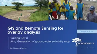
GIS and Remote Sensing for overlay analysis March 22, 2022 Training Day 1 PM / Input data processing (1/3) Dr. Maarten Waterloo www.acaciawater.com
Training program Day Program of activities (AM/PM) Day 1 Introduction to overlay analysis & QGIS / Input data processing (lithology, land use) Tue., March 22nd Day 2 Input data processing (recharge, TWI) / Input data processing (lineament proximity & density) Wed., March 23rd Day 3 Suitability map generation / Automation of suitability mapping Thu., March 24th Day 4 Suitability map styling / Introduction to Google Earth Engine Fri., March 25th Day 5 Introduction to Python Sat., March 26th
Detailed program Day 1 Time Activities 9:00 12:00 Introduction to GIS Introduction to overlay analysis Introduction to QGIS 12:00 13:00 LUNCH BREAK 13:00 16:00 Overlay analysis Step 1 Input layer Lithology Input layer Land use
Overlay analysis - Workflow STEP 0: Data acquisition and basic processing STEP 1: Pre-processing > Clip, resample, reproject, classify, calculate STEP 2: Overlaying > Classes and scores, weights, average suitability STEP 3: Sensitivity analysis
Part 1 Introduction of Overlay Analysis Step 1
Step 1 Principle Output: Overlay layers with uniform resolution, extent and CRS: lithology, land use, recharge, slope, lineaments (x2) Input: CRS (WSG84, UTM 37N), resolution (100 m) Input maps: extent, lithology, DEM, land use, lineaments (x2), precipitation, evapotranspiration Look-up tables (lithology and land use classes) Style definitions
Step 1 Input data Primary data: Lithology Recharge Land use Slope/Topographic Wetness Index (TWI) Lineaments Secondary data: Evapotranspiration Vegetation Index Soil moisture Hydrology (catchments, drainage network, wetness index)
Step 1 Main geo-algorithms Clipping to cluster extent Reprojection and resampling (average or mode) to desired resolution Calculation (recharge, slope, density, proximity) Classification (lithology, land use)
Geo-algorithms Join Shapefile Infiltration coefficient Excel/csv/txt + =
Geo-algorithms Calculation Field calculator Raster calculator Graphical modeler
Part 2 Pre-processing of lithology layer
Pre-processing Lithology layer Source: Harmonized geological map Classification: from 104 => to 7 classes Class Description 1 Loose quaternary sediments, including elluvials and Miocene sediments 2 Rift pyroclastics and rift silicics 3 Upper basalts + Quaternary highland basalts + Rift basalts 4 Lower basalts 5 Limestone + Upper sandstone + Shale + Marl + all other Mesozoics 6 Low grade basement and Adigrate sandstone 7 High grade basement
Lithology layer Procedure 1) Load woreda extent (vector) 2) Load harmonized geological map (vector) 3) Load lithology classes (delimited text) 4) Join table with classes to map using code column > Double click on layer name, then go to Joins menu 5) If joined field is a string (aligned left), then change to number (aligned right) > Field calculator 6) Reproject map to UTM37N, WGS84 (EPSG:32637) > Warp 7) Rasterize reprojected map using 7 classes, set resolution to 100m and extent to woreda extent > Rasterize
Lithology layer Classification Harmonized geological map 7 lithology classes
Part 3 Pre-processing of land use layer
Pre-processing Land use Source: 2016 Sentinel-2A imagery (20 m) Reclassification into 5 classes Class Description 1 Cropland 2 Bush and rangeland 3 Forest 4 Bare soil and degraded land 5 Urban area
Land use layer Procedure 1) Load extent (vector) 2) Load land use data (raster) 3) Reclassify landuse to 5 classes > r.reclass, using overlay/classes/landuse_esa.txt 4) Reproject and resample landuse to UTM37N, WGS84 with resolution 100m and clip to extent (think about resampling method to use) > Warp (Hint: use Mode for resampling methods)
Land use layer Reclassification Reclassified land use (100 m) Land use ESA (20 m)
Thank you for your attention February 26, 2019 van Hogendorpplein 4, 2805 BM Gouda, the Netherlands telephone: +31 (0)182 - 686 424 info@acaciawater.com | www.acaciawater.com