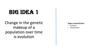
Genetic Variation and Its Role in Evolution
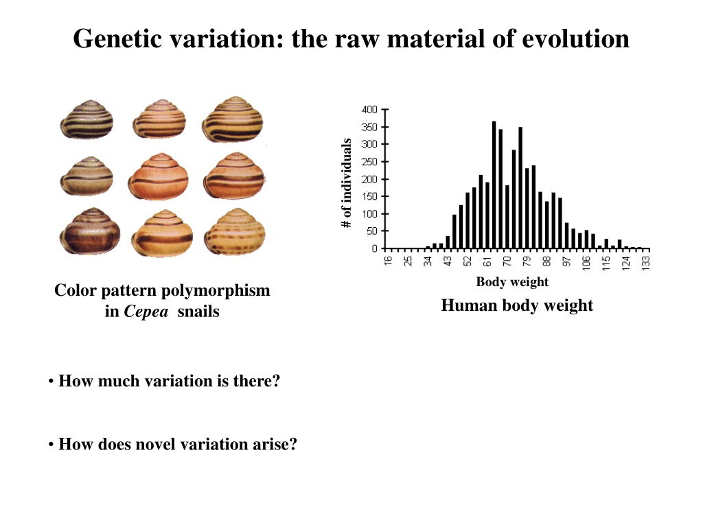

Genetic variation: the raw material of evolution
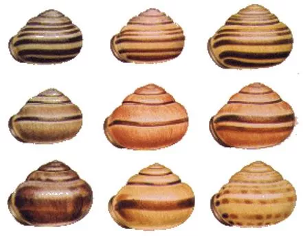
Color pattern polymorphism
in
Cepea
snails

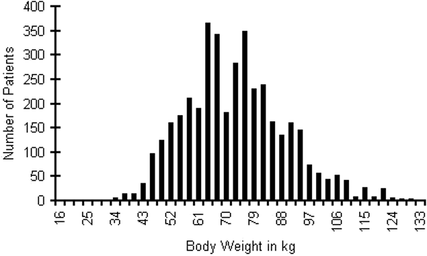
Body weight

# of individuals
Human body weight
•
How much variation is there?
•
How does novel variation arise?

Sources of phenotypic variation
1.
Differences in genotype – Different genotypes produce different
phenotypes
2.
Differences in environment – Different environments produce
different phenotypes
3.
Interactions between genotype and environment – The relative
values of phenotypes produced by different genotypes depend
on the environment
Genetic variation
AA
Aa
aa
Environment 1
Environmental variation
AA
Aa
aa
AA
Aa
aa
Environment 1
Environment 2
Genotype×Environment variation
AA
Aa
aa
AA
Aa
aa
Environment 1
Environment 2
*** Although prevalent in nature, we will ignore the complication of G×E ***
It is GENETIC variation that is essential for evolution
•
Selection can act on purely phenotypic variation
•
But without genetic variation evolution will not occur
Selection
Reproduction
How much genetic variation is there?
1. Statistical analysis of quantitative traits
2. Studies at the molecular level
How much genetic variation is there?
Part I. Statistical analysis of quantitative traits
Body weight
# of individuals
Human body weight
How much of this phenotypic variation is genetic?
Some basic statistics I: The mean
X
i
f
i
Where
n
is the number of different phenotype classes
Basic statistics II: The variance
X
i
f
i
Where
n
is the number of different phenotype classes
Basic statistics II: The variance
X
i
f
i
f
i
Population with variance = 8
Population with variance = 16
Using basic statistics to decompose phenotypic variation
V
P
= V
G
+V
E
Aa
AA
aa
Genetic Variance
f
i
X
i
E1
E2
E3
X
i
Environmental Variance
+
X
i
f
i
Phenotypic Variance
Genetic variation can be further decomposed
V
G
= V
A
+V
I
+V
D
Additive Genetic Variance
f
i
X
i
X
i
Epistasis and Dominance Variance
+
X
i
f
i
Genotypic Variance
What mechanisms contribute to each component?
Additive genetic variance (V
A
) – Due to the
additive effects of alleles
Dominance variance (V
D
) – Due to dominance
Interaction variance (V
I
) – Due to epistasis
It is
additive genetic variance
that determines the
resemblance of parents and offspring
How do we know how much additive genetic variation exists within a population?
♂
♀
♂
♀
Additvity
Epistasis or Dominance
Offspring need not look like parents!
The proportion of phenotypic variation that is genetic can
be estimated by calculating “heritability”
•
Broad sense heritability – Measures the proportion of phenotypic variation
that is genetic
•
Narrow sense heritability
– Measures the proportion of phenotypic variation
attributable to the additive action of genes. This is the measure relevant to
N.S.
How can we measure narrow sense heritability?
One possibility is a parent-offspring regression
Offspring value (z
Offspring
)
Mid parent value (z
Parent
)
•
The slope of the linear regression is an estimate of heritability
One possibility is a parent-offspring regression
Offspring value
Perfectly heritable –
Slope is 1.0
High heritability –
Slope is 0.8685
Low heritability –
Slope is 0.0756
Offspring value
Offspring value
Mid parent value
How heritable are most traits?
After Falconer (1981)
For almost any trait ever measured, there is abundant additive genetic variation!
A limitation of the statistical approach
Can never accurately reveal how many genetic loci are responsible for
observed levels of variation
vs.
How much genetic variation is there?
Part II: Molecular variability
•
Prior to 1966, it was generally assumed that populations were,
in large part, genetically uniform
•
In 1966, two landmark papers (Lewinton and Hubby, 1966;
Harris, 1966) turned this conventional wisdom on its head,
demonstrating an abundance of
GENETIC POLYMORPHISM
So what did these landmark studies really show?
Genetic polymorphism
– The presence of two or more alleles in a population,
with the rarer allele having a frequency greater than .01.
Using protein gel electrophoresis, these studies showed that roughly 1/3 of all
loci are polymorphic in both humans and
Drosophila
.
Separates protein
variants (alleles)
by size and charge
In this example, there
are 5 alleles
Subsequent studies found the same thing!
Source: Futuyma,
Evolutionary Biology, 3’rd Edition
Suggests that almost every individual in a sexually
reproducing species is genetically unique!
•
Even with only two alleles per locus, the estimated 3000 polymorphic loci
in humans could generate 3
3000
= 10
1431
different genotypes!
The bottom line:
No matter how you cut it,
there is abundant genetic variation WITHIN populations,
and thus ample opportunity for selection to act
Assessing genetic variation and Hardy-Weinberg I:
a practice problem
The scenario:
A group of biologists was studying a population of elk in an effort to
quantify genetic variation at disease resistance locus. Through DNA sequencing, the
biologists have determined that there are two alleles at this locus,
A
and
a
.
Sequencing analysis of many individuals has also allowed the frequency of the alleles
and the corresponding diploid genotypes to be estimated
The data:
Frequency of the
A
allele is
p
= 0.4
Frequency of the
a
allele is
q
= ?
Frequency of the
AA
genotype is: 0.06
Frequency of the
Aa
genotype is: 0.80
Frequency of the
aa
genotype is: 0.14
The question:
Is this population in Hardy-Weinberg Equilibrium? Justify your response.
Increasing the scale:
Genetic variation among populations
aa
aa
aa
aa
Aa
AA
aa
AA
Aa
AA
Aa
Aa
AA
AA
AA
AA
AA
AA
AA
AA
aa
aa
Genetic variation within a single population
Genetic variation among populations
Genetic variation among populations
Genetic variation in human resistance to Malaria
Increasing the scale: Genetic variation among species
Chinook < 100 lbs
Coho < 26 lbs
Chum < 32 lbs
Pink < 12 lbs
Sockeye < 16 lbs
These different species are genetically differentiated with respect to adult size
We now know that genetic variation is hierarchical
AA
AA
Aa
Aa
Aa
aa
aa
aa
AA
A
B
Aa
AA
AA
AA
Aa
AA
AA
AA
Aa
Aa
Aa
a
B
aa
aa
Aa
aA
aa
Aa
aa
aa
aa
aa
BB
bb
B
A
BB
Bb
Bb
a
B
BA
Bb
Bb
Bb
Bb
bb
bb
bb
bb
bb
Bb
bb
bb
Bb
bb
bb
bb
BB
BB
BB
Bb
BB
BB
Bb
B
a
Species A
Species B
Populations
An applied problem: genetic variation and conservation
Sockeye Salmon
Redfish Lake, Idaho
Populations vs. Species:
Which is more relevant?
Assessing genetic variation and Hardy-Weinberg II:
a practice problem
The scenario:
A group of biologists is studying a population of flowers where flower
color is controlled by a single diploid locus with two alleles. Individuals with
genotype
AA
make white flowers, individuals with genotype
Aa
make red flowers,
and individuals with genotype
aa
make red flowers.
The data:
Frequency of the white flowers is
f(white)
= 0.4
Frequency of red flowers is f(red) = ?
The questions:
1.
Which allele,
A
or
a
is dominant?
2.
Assuming that this population is in Hardy-Weinberg Equilibrium, what is the
frequency of the
A
allele?
3.
Assuming that this population is in Hardy-Weinberg Equilibrium, what is the
frequency of the
a
allele?
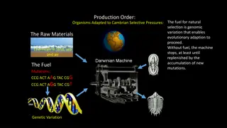
Where does genetic variation come from?
1. Mutation – An alteration of a DNA sequence that is inherited
2. Recombination – The formation of gametes with combinations
of alleles different from those that united to form the individual that
produced them.
3. Gene flow – The incorporation of genes into the gene pool of one
population from one or more other populations.
4. Hybridization – The incorporation of genes into the gene pool of one
species from another species.
Important facts about mutation
•
Mutations are RANDOM with respect to fitness
•
Only mutations that are inherited (germline) are relevant to evolution
Estimating the mutation rate
•
Direct methods – Simply counting new mutations
•
Statistical methods – Based on increases in phenotypic variance
Direct estimation of the mutation rate
G =
1
G =
2
50,000 flies all homozygous for the (hypothetical) recessive red eye allele (A)
50,000 flies but now 1 has white eyes indicating genotype (Aa)
We could then estimate that the per locus mutation rate as 1/100,000 = .00001
AA
Aa
Implications of these estimates for mutation rates
•
As a gross average, the per locus mutation rate is 10
-6
- 10
-5
mutations per gamete per generation.
•
As a gross average, humans have 150,000 functional genes
•
10
-5
(150,000) = 1.5
This suggests that EVERY gamete carries a new, phenotypically
detectable mutation somewhere in its genome!!!
Spontaneous mutation rates of specific genes
detected by phenotypic effects
Source: Evolutionary analysis: third edition. Freeman and Herron.
Statistical estimation of new mutational genetic variance
Inbreed until all additive
genetic variance for some trait of
interest is lost
Mate at random and
measure heritability
It would then take only 100 generations for
h
2
to equal .1!
Tribolium
(flour beetle)
length
h
2
= V
A
/ V
P
= .001
h
2
= V
A
/ V
P
= 0
What effect do mutations have on fitness?
Fitness of mutants
Frequency
Below average
Above average
Although we know very little, we know that new mutations are generally
deleterious
Recombination as a source of variation
Recombination generates new COMBINATIONS of genes
AB/AB
AB/ab
ab/ab
ab/AB
AB
aB
Ab
ab
Recombination absent
Recombination present
Zygotes
AB/AB
AB/ab
ab/ab
ab/AB
Zygotes
Gametes
AB
ab
Gametes
Fusion
Meiosis
(no recombination)
Meiosis
(recombination)
Fusion
AB/AB
AB/ab
ab/ab
ab/AB
Zygotes
AB/AB
AB/ab
ab/ab
ab/AB
Zygotes
aB/AB
Ab/AB
Ab/aB
aB/Ab
Gene flow as a source of variation
Population 1
Population 2
AA
AA
AA
AA
AA
aa
aa
aa
aa
aa
Population 1
Population 2
AA
AA
aa
Aa
aA
AA
aa
aA
aa
Aa
Gene Flow
V
G
= 0
V
G
= 0
V
G
> 0
V
G
> 0
Hybridization as a source of genetic variation
AA
AA
AA
AA
AA
aA
Aa
Aa
aA
Aa
aa
aa
aa
aa
aa
•
Hybridization reshuffles genes between species
•
Often has dramatic phenotypic effects
•
IF
offspring are viable and fertile, hybridization
can be an important source of new genetic
variation
Hybridization as a source of genetic variation
Aquilegia formosa
Lower elevations (6000-10,000 ft)
Aquilegia pubescens
High elevations (10,000-13,000 ft).
Both species grow in the Sierra Nevada mountains of California
Scott
Hodges
Scott
Hodges
Hybridization as a source of genetic variation
Formosa - Pubescens hybrid zone
Summary
•
There is abundant genetic variation in natural populations
•
Mutation is the ultimate source of genetic variation
•
Recombination, gene flow, and hybridization redistribute
genetic variation
Practice Problem
You are studying a population of Steelhead Trout and would like to know to what extent body
mass is heritable. To this end, you measured the body mass of male and female Steelhead as
well as the body mass of their offspring. Use the data from this experiment (below) to estimate
the heritability of body mass in this population of Steelhead.
Genetic variation is crucial for evolution, providing the raw material for adaptation and species diversity. Phenotypic variation can arise from differences in genotype, environment, or their interaction. Studying genetic variation through statistical analysis and at the molecular level helps us unravel its extent and impact on traits. Without genetic variation, evolution would be constrained, emphasizing its essential role in shaping biological diversity.

Download Presentation

Please find below an Image/Link to download the presentation.
The content on the website is provided AS IS for your information and personal use only. It may not be sold, licensed, or shared on other websites without obtaining consent from the author.If you encounter any issues during the download, it is possible that the publisher has removed the file from their server.
You are allowed to download the files provided on this website for personal or commercial use, subject to the condition that they are used lawfully. All files are the property of their respective owners.
The content on the website is provided AS IS for your information and personal use only. It may not be sold, licensed, or shared on other websites without obtaining consent from the author.
E N D
Presentation Transcript
Genetic variation: the raw material of evolution # of individuals Body weight Human body weight Color pattern polymorphism in Cepea snails How much variation is there? How does novel variation arise?
Sources of phenotypic variation 1. Differences in genotype Different genotypes produce different phenotypes 2. Differences in environment Different environments produce different phenotypes 3. Interactions between genotype and environment The relative values of phenotypes produced by different genotypes depend on the environment
Genetic variation Environment 1 aa AA Aa
Environmental variation Environment 1 aa AA Aa Environment 2 aa AA Aa
GenotypeEnvironment variation Environment 1 aa AA Aa Environment 2 aa AA Aa *** Although prevalent in nature, we will ignore the complication of G E ***
It is GENETIC variation that is essential for evolution Selection can act on purely phenotypic variation Selection But without genetic variation evolution will not occur Reproduction
How much genetic variation is there? 1. Statistical analysis of quantitative traits 5 y = 0.8685x + 0.2704 4 3 2 1 1 2 3 4 5 2. Studies at the molecular level
How much genetic variation is there? Part I. Statistical analysis of quantitative traits # of individuals Body weight Human body weight How much of this phenotypic variation is genetic?
Some basic statistics I: The mean = i 1 n = x f iX i 1 0.75 fi 0.5 0.25 0 4 8 12 Xi = ) 8 ( 5 . + + = 25 . ) 4 ( 25 . 12 ( ) 8 x Where n is the number of different phenotype classes
Basic statistics II: The variance n = i = 2) ( V f X x i i 1 1 0.75 fi 0.5 0.25 0 4 8 12 Xi = ) 8 8 ( 5 . + ) 8 + ) 8 = 2 2 2 25 . 4 ( 25 . 12 ( 8 V Where n is the number of different phenotype classes
Basic statistics II: The variance 1 Population with variance = 8 0.75 0 ( 0 = ) 8 + ) 8 8 ( 5 . + ) 8 + 2 2 2 25 . 4 ( V fi ) 8 ( 0 + ) 8 = 2 2 25 . 12 ( 16 8 0.5 0.25 0 0 4 8 12 16 1 Population with variance = 16 0.75 = ) 8 + ) 8 + ) 8 + 2 2 2 0625 . 0 ( 25 . 4 ( 375 . 8 ( V fi 0.5 ) 8 + ) 8 = 2 2 25 . 12 ( 0625 . 16 ( 16 0.25 0 0 4 8 12 16 Xi
Using basic statistics to decompose phenotypic variation VP = VG+VE Genetic Variance Environmental Variance 1 1 + 0.75 0.75 Aa E2 fi 0.5 0.5 aa E1 AA E3 0.25 0.25 0 0 0 4 8 12 16 0 -1 0 1 0 Xi Xi Phenotypic Variance 1 0.75 fi 0.5 0.25 0 0 4 8 12 16 Xi
Genetic variation can be further decomposed VG = VA+VI+VD Additive Genetic Variance Epistasis and Dominance Variance 1 1 + 0.75 0.75 fi 0.5 0.5 0.25 0.25 0 0 0 4 8 12 16 0 -1 0 1 0 Xi Xi Genotypic Variance 1 0.75 fi 0.5 0.25 0 0 4 8 12 16 Xi
What mechanisms contribute to each component? Additive genetic variance (VA) Due to the additive effects of alleles Genotype Phenotype AA 2 Aa 1 aa 0 Dominance variance (VD) Due to dominance Genotype Phenotype AA 2 Aa 1 aa 2 Interaction variance (VI) Due to epistasis Genotype Phenotype AA (BB) 2 AA (Bb) 1 AA (bb) 2
It is additive genetic variance that determines the resemblance of parents and offspring Additvity Epistasis or Dominance Offspring need not look like parents! How do we know how much additive genetic variation exists within a population?
The proportion of phenotypic variation that is genetic can be estimated by calculating heritability Broad sense heritability Measures the proportion of phenotypic variation that is genetic = + = 2 /( ) / H V V V V V B G G E G P Narrow sense heritability Measures the proportion of phenotypic variation attributable to the additive action of genes. This is the measure relevant to N.S. = + + + 2 N /( ) h V V V V V A A I D E How can we measure narrow sense heritability?
One possibility is a parent-offspring regression The slope of the linear regression is an estimate of heritability Offspring value (zOffspring) 5 y = 0.8685x + 0.2704 4 [ , ] Cov z z Parent z V Offspring h = 2 3 [ ] Parent 2 1 1 2 3 4 5 Mid parent value (zParent) )( ) n ( = z z z z , , Parent i Parent Offspring i Offspring = 1 [ , ] i Cov z z Parent Offspring n
One possibility is a parent-offspring regression 5 y = x Offspring value 4 Perfectly heritable Slope is 1.0 3 2 1 1 2 3 4 5 5 Offspring value y = 0.8685x + 0.2704 4 High heritability Slope is 0.8685 3 2 1 1 2 3 4 5 5 Offspring value 4 y = 0.0756x + 2.0683 Low heritability Slope is 0.0756 3 2 1 0 2 4 6 Mid parent value
How heritable are most traits? Trait Heritability Milk Yield in Cattle .3 Body length in pigs .5 Litter size in pigs .15 Wool length in sheep .55 Egg weight in chickens .6 Age at first laying In chickens .5 Tail length in mice .6 Litter size in mice .15 After Falconer (1981) For almost any trait ever measured, there is abundant additive genetic variation!
A limitation of the statistical approach vs. Can never accurately reveal how many genetic loci are responsible for observed levels of variation
How much genetic variation is there? Part II: Molecular variability Prior to 1966, it was generally assumed that populations were, in large part, genetically uniform In 1966, two landmark papers (Lewinton and Hubby, 1966; Harris, 1966) turned this conventional wisdom on its head, demonstrating an abundance of GENETIC POLYMORPHISM
So what did these landmark studies really show? Genetic polymorphism The presence of two or more alleles in a population, with the rarer allele having a frequency greater than .01. Separates protein variants (alleles) by size and charge In this example, there are 5 alleles Using protein gel electrophoresis, these studies showed that roughly 1/3 of all loci are polymorphic in both humans and Drosophila.
Subsequent studies found the same thing! Source: Futuyma, Evolutionary Biology, 3 rd Edition
Suggests that almost every individual in a sexually reproducing species is genetically unique! Even with only two alleles per locus, the estimated 3000 polymorphic loci in humans could generate 33000 = 101431 different genotypes!
The bottom line: No matter how you cut it, there is abundant genetic variation WITHIN populations, and thus ample opportunity for selection to act
Assessing genetic variation and Hardy-Weinberg I: a practice problem The scenario: A group of biologists was studying a population of elk in an effort to quantify genetic variation at disease resistance locus. Through DNA sequencing, the biologists have determined that there are two alleles at this locus, A and a. Sequencing analysis of many individuals has also allowed the frequency of the alleles and the corresponding diploid genotypes to be estimated The data: Frequency of the A allele is p = 0.4 Frequency of the a allele is q = ? Frequency of the AA genotype is: 0.06 Frequency of the Aa genotype is: 0.80 Frequency of the aa genotype is: 0.14 The question: Is this population in Hardy-Weinberg Equilibrium? Justify your response.
Increasing the scale: Genetic variation among populations Genetic variation within a single population Aa Aa AA AA aaAA Aa Aa AA Genetic variation among populations AA AA aa AA aa AA aa AA AA aa aa AA aa
Genetic variation among populations Genetic variation in human resistance to Malaria
Increasing the scale: Genetic variation among species Chum < 32 lbs Chinook < 100 lbs Coho < 26 lbs Pink < 12 lbs Sockeye < 16 lbs These different species are genetically differentiated with respect to adult size
We now know that genetic variation is hierarchical aa Bb Aa BB aA BB aa bb AA bb aa BB AA Bb Aa Bb aa BB Aa bb aa aa Aa Ba BB bb aB bb aa Aa bb Bb aa aB AA BB Aa bb AA bb Aa BA AA Bb Aa BB BA AB Bb aa Bb Aa Bb aa Aa Bb AA AA Bb AA bb AA bb bb Populations Species B Species A
An applied problem: genetic variation and conservation Sockeye Salmon Redfish Lake, Idaho Populations vs. Species: Which is more relevant?
Assessing genetic variation and Hardy-Weinberg II: a practice problem The scenario: A group of biologists is studying a population of flowers where flower color is controlled by a single diploid locus with two alleles. Individuals with genotype AA make white flowers, individuals with genotype Aa make red flowers, and individuals with genotype aa make red flowers. The data: Frequency of the white flowers is f(white) = 0.4 Frequency of red flowers is f(red) = ? The questions: 1. Which allele, A or a is dominant? 2. Assuming that this population is in Hardy-Weinberg Equilibrium, what is the frequency of the A allele? 3. Assuming that this population is in Hardy-Weinberg Equilibrium, what is the frequency of the a allele?
Where does genetic variation come from? 1. Mutation An alteration of a DNA sequence that is inherited 2. Recombination The formation of gametes with combinations of alleles different from those that united to form the individual that produced them. 3. Gene flow The incorporation of genes into the gene pool of one population from one or more other populations. 4. Hybridization The incorporation of genes into the gene pool of one species from another species.
Important facts about mutation Mutations are RANDOM with respect to fitness Only mutations that are inherited (germline) are relevant to evolution
Estimating the mutation rate Direct methods Simply counting new mutations Statistical methods Based on increases in phenotypic variance
Direct estimation of the mutation rate AA G = 1 50,000 flies all homozygous for the (hypothetical) recessive red eye allele (A) Aa G = 2 50,000 flies but now 1 has white eyes indicating genotype (Aa) We could then estimate that the per locus mutation rate as 1/100,000 = .00001
Implications of these estimates for mutation rates As a gross average, the per locus mutation rate is 10-6 - 10-5 mutations per gamete per generation. As a gross average, humans have 150,000 functional genes 10-5 (150,000) = 1.5 This suggests that EVERY gamete carries a new, phenotypically detectable mutation somewhere in its genome!!!
Spontaneous mutation rates of specific genes detected by phenotypic effects Estimates of mutation rates (per genome, per generation) Single celled organisms Species Taxonomic group Bacteria Archaea Fungi Fungi Multicellular organisms Species Taxonomic group Roundworms Insects Mammals Mammals Number of mutations 0.0025 0.0018 0.0030 0.0027 E. Coli S. acidocaldarius N. crassa S. cerevisiae Number of mutations 0.0360 0.1400 0.9000 1.6000 C. elegans D. Melanogaster M. Musculus H. sapiens Source: Evolutionary analysis: third edition. Freeman and Herron.
Statistical estimation of new mutational genetic variance 0.35 0.8 0.3 0.7 0.25 0.6 0.2 0.5 0.4 0.15 0.3 0.1 Inbreed until all additive genetic variance for some trait of interest is lost 0.2 0.05 0.1 0 0 0 1 2 3 4 5 6 0 1 2 3 4 5 6 Tribolium (flour beetle) length h2 = VA / VP= 0 0.7 Mate at random and measure heritability 0.6 0.5 0.4 0.3 0.2 0.1 0 0 1 2 3 4 5 6 h2 = VA / VP = .001 It would then take only 100 generations for h2 to equal .1!
What effect do mutations have on fitness? Below average Above average 0.18 0.16 0.14 0.12 Frequency 0.1 0.08 0.06 0.04 0.02 0 0 0.1 0.2 0.3 0.4 0.5 0.6 0.7 Fitness of mutants 0.8 0.9 1 1.1 1.2 1.3 1.4 1.5 Although we know very little, we know that new mutations are generally deleterious
Recombination as a source of variation Recombination absent Recombination present Zygotes Zygotes ab/AB ab/AB AB/AB AB/AB AB/ab AB/ab ab/ab ab/ab Meiosis Meiosis (no recombination) (recombination) Gametes Gametes ab aB Ab AB AB ab Fusion Fusion Zygotes Zygotes Ab/AB aB/AB ab/AB ab/AB Ab/aB AB/AB AB/ab aB/Ab ab/ab AB/ab AB/AB ab/ab Recombination generates new COMBINATIONS of genes
Gene flow as a source of variation VG = 0 VG = 0 aa AA AA aa aa AA AA aa aa AA Population 1 Population 2 VG > 0 VG > 0 AA Aa AA aa Gene Flow aA aA AA Aa aa aa Population 1 Population 2
Hybridization as a source of genetic variation 694px-Horse_in_field aa AA AA aa aa AA AA aa aa AA Hybridization reshuffles genes between species Often has dramatic phenotypic effects IF offspring are viable and fertile, hybridization can be an important source of new genetic variation aA Aa Aa aAAa
Hybridization as a source of genetic variation Scott Hodges Scott Hodges Aquilegia formosa Lower elevations (6000-10,000 ft) Aquilegia pubescens High elevations (10,000-13,000 ft). Both species grow in the Sierra Nevada mountains of California
Hybridization as a source of genetic variation Formosa - Pubescens hybrid zone
Summary There is abundant genetic variation in natural populations Mutation is the ultimate source of genetic variation Recombination, gene flow, and hybridization redistribute genetic variation
Practice Problem You are studying a population of Steelhead Trout and would like to know to what extent body mass is heritable. To this end, you measured the body mass of male and female Steelhead as well as the body mass of their offspring. Use the data from this experiment (below) to estimate the heritability of body mass in this population of Steelhead. Maternal Body Mass (Kg) Paternal Body Mass (Kg) Average Offspring Body Mass (Kg) 2.1 2.5 1.9 2.2 1.8 2.4 2.3 2.6 2.9 3.1 2.8 2.7 2.4 2.9 2.3 2.5 2.7 2.4 2.3 2.2 2.7