Fundamentals of Bayes Theorem and Classification
Bayes Theorem is a powerful tool for probabilistic reasoning and classification tasks. It involves deriving posterior probabilities based on prior knowledge and observed data. This technique is essential in making predictions and maximizing the accuracy of classification models. Nave Bayes Classifier simplifies the computation process by assuming attribute independence, making it efficient for various datasets. Explore the basics of Bayes Theorem, prediction, classification, and Nave Bayes Classifier through practical examples and understand the core concepts behind these statistical methods.

Download Presentation

Please find below an Image/Link to download the presentation.
The content on the website is provided AS IS for your information and personal use only. It may not be sold, licensed, or shared on other websites without obtaining consent from the author.If you encounter any issues during the download, it is possible that the publisher has removed the file from their server.
You are allowed to download the files provided on this website for personal or commercial use, subject to the condition that they are used lawfully. All files are the property of their respective owners.
The content on the website is provided AS IS for your information and personal use only. It may not be sold, licensed, or shared on other websites without obtaining consent from the author.
E N D
Presentation Transcript
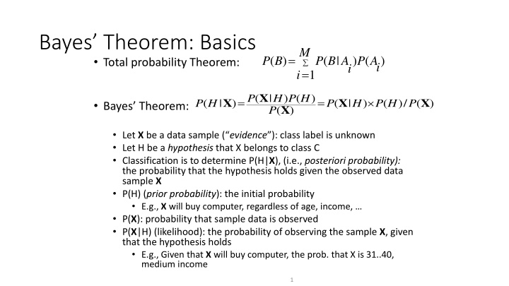
Bayes Theorem: Basics M = = ( ) ( | ) ( ) P B P B A P A Total probability Theorem: i i 1 i X ( | P ) ( ) P H P H = = X X X ( | ) ( | ) ( / ) ( ) P H P H P H P Bayes Theorem: X ( ) Let X be a data sample ( evidence ): class label is unknown Let H be a hypothesis that X belongs to class C Classification is to determine P(H|X), (i.e., posteriori probability): the probability that the hypothesis holds given the observed data sample X P(H) (prior probability): the initial probability E.g., X will buy computer, regardless of age, income, P(X): probability that sample data is observed P(X|H) (likelihood): the probability of observing the sample X, given that the hypothesis holds E.g., Given that X will buy computer, the prob. that X is 31..40, medium income 1
Prediction Based on Bayes Theorem Given training data X, posteriori probability of a hypothesis H, P(H|X), follows the Bayes theorem X ( | P ) ( ) P H P H = = X X X ( | ) ( | ) ( / ) ( ) P H P H P H P X ( ) Informally, this can be viewed as posteriori = likelihood x prior/evidence Predicts X belongs to Ciiff the probability P(Ci|X) is the highest among all the P(Ck|X) for all the k classes Practical difficulty: It requires initial knowledge of many probabilities, involving significant computational cost 2
Classification is to Derive the Maximum Posteriori Let D be a training set of tuples and their associated class labels, and each tuple is represented by an n-D attribute vector X = (x1, x2, , xn) Suppose there are m classes C1, C2, , Cm. Classification is to derive the maximum posteriori, i.e., the maximal P(Ci|X) This can be derived from Bayes theorem X ( | P ) ( ) P C P C i i = X ( | ) P C i X ( ) Since P(X) is constant for all classes, only X = X ( | ) ( | ) ( ) P C P C P C i i i needs to be maximized 3
Nave Bayes Classifier A simplified assumption: attributes are conditionally independent (i.e., no dependence relation between attributes): n P Ci = = = X ( | ) ( | ) ( | ) ( | ) ... ( | ) P P P P x Ci x Ci x Ci x Ci 1 2 k n 1 k This greatly reduces the computation cost: Only counts the class distribution If Akis categorical, P(xk|Ci) is the # of tuples in Cihaving value xkfor Akdivided by |Ci, D| (# of tuples of Ciin D) If Akis continous-valued, P(xk|Ci) is usually computed based on Gaussian distribution with a mean and standard deviation 2 ( ) x 1 and P(xk|Ci) is = 2 ( , , ) g x e 2 2 = X ( | ) ( , , ) P g kx Ci C C i i 4
Nave Bayes Classifier: Training Dataset age income student credit_rating buys_computer <=30 high no fair no Class: <=30 high no excellent no 31 40 high no fair yes C1:buys_computer = yes C2:buys_computer = no >40 medium no fair yes >40 low yes fair yes >40 low yes excellent no Data to be classified: X = (age <=30, income = medium, student = yes, credit_rating = fair) 31 40 low yes excellent yes <=30 medium no fair no <=30 low yes fair yes >40 medium yes fair yes <=30 medium yes excellent yes X buy computer? 31 40 medium No excellent yes 31 40 high Yes fair yes >40 medium No excellent no 5
age <=30 <=30 31 40 >40 >40 >40 31 40 <=30 <=30 >40 <=30 31 40 31 40 >40 income high high high medium no low low low medium no low medium yes medium yes medium no high medium no student credit_rating buys_computer no fair no excellent no fair fair yes fair yes excellent yes excellent fair yes fair fair excellent excellent yes fair excellent no no yes yes yes no yes no yes yes yes yes yes no Na ve Bayes Classifier: An Example P(Ci): P(buys_computer = yes ) = 9/14 = 0.643 P(buys_computer = no ) = 5/14= 0.357 Compute P(X|Ci) for each class P(age = <=30 | buys_computer = yes ) = 2/9 = 0.222 P(age = <= 30 | buys_computer = no ) = 3/5 = 0.6 P(income = medium | buys_computer = yes ) = 4/9 = 0.444 P(income = medium | buys_computer = no ) = 2/5 = 0.4 P(student = yes | buys_computer = yes) = 6/9 = 0.667 P(student = yes | buys_computer = no ) = 1/5 = 0.2 P(credit_rating = fair | buys_computer = yes ) = 6/9 = 0.667 P(credit_rating = fair | buys_computer = no ) = 2/5 = 0.4 X = (age <= 30 , income = medium, student = yes, credit_rating = fair) P(X|Ci) : P(X|buys_computer = yes ) = 0.222 x 0.444 x 0.667 x 0.667 = 0.044 P(X|buys_computer = no ) = 0.6 x 0.4 x 0.2 x 0.4 = 0.019 P(X|Ci)*P(Ci) : P(X|buys_computer = yes ) * P(buys_computer = yes ) = 0.028 P(X|buys_computer = no ) * P(buys_computer = no ) = 0.007 Therefore, X belongs to class ( buys_computer = yes ) 6
Tahapan Algoritma Nave Bayes 1. Baca Data Training 2. Hitung jumlah class 3. Hitung jumlah kasus yang sama dengan class yang sama 4. Kalikan semua nilai hasil sesuai dengan data X yang dicari class-nya 7
Teorema Bayes X ( | P ) ( ) P H P H = = X X X ( | ) ( | ) ( / ) ( ) P H P H P H P X ( ) X H Data dengan class yang belum diketahui Hipotesis data X yang merupakan suatu class yang lebih spesifik P (H|X) Probabilitas hipotesis H berdasarkan kondisi X (posteriori probability) P (H) Probabilitas hipotesis H (prior probability) P (X|H) Probabilitas X berdasarkan kondisi pada hipotesis H P (X) Probabilitas X 9
2. Hitung jumlah class/label Terdapat 2 class dari data training tersebut, yaitu: C1 (Class 1) Play = yes 9 record C2 (Class 2) Play = no 5 record Total = 14 record Maka: P (C1) = 9/14 = 0.642857143 P (C2) = 5/14 = 0.357142857 Pertanyaan: Data X = (outlook=rainy, temperature=cool, humidity=high, windy=true) Main golf atau tidak? 10
3. Hitung jumlah kasus yang sama dengan class yang sama Untuk P(Ci) yaitu P(C1) dan P(C2) sudah diketahui hasilnya di langkah sebelumnya. Selanjutnya Hitung P(X|Ci) untuk i = 1 dan 2 P(outlook= sunny |play= yes )=2/9=0.222222222 P(outlook= sunny |play= no )=3/5=0.6 P(outlook= overcast |play= yes )=4/9=0.444444444 P(outlook= overcast |play= no )=0/5=0 P(outlook= rainy |play= yes )=3/9=0.333333333 P(outlook= rainy |play= no )=2/5=0.4 11
3. Hitung jumlah kasus yang sama dengan class yang sama Jika semua atribut dihitung, maka didapat hasil akhirnya seperti berikut ini: Atribute Parameter Outlook value=sunny Outlook value=cloudy Outlook value=rainy Temperature value=hot Temperature value=mild Temperature value=cool Humidity value=high Humidity value=normal Windy value=false Windy value=true No 0.6 0.0 0.4 0.4 0.4 0.2 0.8 0.2 0.4 0.6 Yes 0.2222222222222222 0.4444444444444444 0.3333333333333333 0.2222222222222222 0.4444444444444444 0.3333333333333333 0.3333333333333333 0.6666666666666666 0.6666666666666666 0.3333333333333333 12
4. Kalikan semua nilai hasil sesuai dengan data X yang dicari class-nya Pertanyaan: Data X = (outlook=rainy, temperature=cool, humidity=high, windy=true) Main Golf atau tidak? Kalikan semua nilai hasil dari data X P(X|play= yes ) = 0.333333333* 0.333333333* 0.333333333*0.333333333 = 0.012345679 P(X|play= no ) = 0.4*0.2*0.8*0.6=0.0384 P(X|play= yes )*P(C1) = 0.012345679*0.642857143 = 0.007936508 P(X|play= no )*P(C2) = 0.0384*0.357142857 = 0.013714286 Nilai no lebih besar dari nilai yes maka class dari data X tersebut adalah No 13
Avoiding the Zero-Probability Problem Na ve Bayesian prediction requires each conditional prob. be non-zero. Otherwise, the predicted prob. will be zero = Ci X P ) | ( n = ( | ) P 1 xk Ci k Ex. Suppose a dataset with 1000 tuples, income=low (0), income= medium (990), and income = high (10) Use Laplacian correction (or Laplacian estimator) Adding 1 to each case Prob(income = low) = 1/1003 Prob(income = medium) = 991/1003 Prob(income = high) = 11/1003 The corrected prob. estimates are close to their uncorrected counterparts 14
Nave Bayes Classifier: Comments Advantages Easy to implement Good results obtained in most of the cases Disadvantages Assumption: class conditional independence, therefore loss of accuracy Practically, dependencies exist among variables, e.g.: Hospitals Patients Profile: age, family history, etc. Symptoms: fever, cough etc., Disease: lung cancer, diabetes, etc. Dependencies among these cannot be modeled by Na ve Bayes Classifier How to deal with these dependencies? Bayesian Belief Networks 15