Exploring Time-Frequency Analysis Techniques

An Introduction to Time-Frequency Analysis Advisor : Jian-Jiun Ding, Ph. D. Presenter : Ke-Jie Liao Taiwan ROC Taipei National Taiwan University GICE DISP Lab MD531

Outline Introduction STFT Rectangular STFT Gabor Transform Wigner Distribution Function Motions on the Time-Frequency Distribution FRFT LCT Applications on Time-Frequency Analysis Signal Decomposition and Filter Design Sampling Theory Modulation and Multiplexing 2

Introduction Frequency? Another way to consider things. Frequency related applications FDM Sampling Filter design , etc . 3

Introduction Conventional Fourier transform 1-D Totally losing time information Suitable for analyzing stationary signal ,i.e. frequency does not vary with time. [1] 4

Introduction Time-frequency analysis Mostly originated form FT Implemented using FFT [1] 5

Short Time Fourier Transform Modification of Fourier Transform Sliding window, mask function, weighting function Mathematical expression ( ) ( , ) ( ) X t f x w t w(t) = = ( )} 2 j f { ( ) e d F w t x Reversing Shifting FT 6

Short Time Fourier Transform Requirements of the mask function w(t) is an even function. i.e. w(t)=w(-t). max(w(t))=w(0),w(t1) when |t| is large. An example of window functions w(t2) if |t1|<|t2|. w t ( ) 0 t Window width K 7

Short Time Fourier Transform Requirements of the mask function w(t) is an even function. i.e. w(t)=w(-t). max(w(t))=w(0),w(t1) when |t| is large. An illustration of evenness of mask functions w(t2) if |t1|<|t2|. w t ( ) 0 Mask Signal t0 8

Short Time Fourier Transform Effect of window width K Controlling the time resolution and freq. resolution. Small K Better time resolution, but worse in freq. resolution Large K Better freq. resolution, but worse in time resolution 9

Short Time Fourier Transform The time-freq. area of STFTs are fixed f f K decreases t t 10

Rectangular STFT Rectangle as the mask function Uniform weighting Definition Forward 1 + t B = ( ) 2B 2 j f ( , ) X t f x e d t B Inverse = where 2 j ft ( ) x t ( , ) X t f e df + t B t t B 1 1 11

Rectangular STFT Examples of Rectangular STFTs cos(4 ) ,0 ( ) cos(2 ) ,10 cos( ) t f 2 ,0 1 ,10 0.5 10 20 10 t t t = = ( ) f t t 20 30 x t t t i ,20 30 t ,20 t f B=0.25 B=0.5 2 1 0 2 1 0 t t 30 0 10 20 30 0 10 20 12

Rectangular STFT Examples of Rectangular STFTs cos(4 ) ,0 ( ) cos(2 ) ,10 cos( ) t f 2 ,0 1 ,10 0.5 10 20 t 10 t t t t = = ( ) f t t 20 30 x t t i ,20 30 ,20 t f B=1 B=3 2 1 0 2 1 0 t t 30 0 10 20 30 0 10 20 13

Rectangular STFT Properties of rec-STFTs Linearity = + ( ) ( , ) H t f ( ) x t = ( ) y t h t + ( , ) Y t f ( , ) X t f Shifting t B + = 2 2 j f j f ( ) ( , ) f e x e d X t 0 0 0 t B Modulation t B + = 2 2 j f j f [ ( ) x ] ( , ) e e d X t f f 0 0 t B 14

Rectangular STFT Properties of rec-STFTs Integration + ( ), x v v B t v B = 2 j fv ( , ) X t f e df 0 , otherwise Power integration t B + = ( ) ( ) * * ( , ) X t f ( , ) Y t f df x y d t B Energy sum = * * ( , ) X t f ( , ) ( ) ( ) Y t f dfdt B x y d 15

Gabor Transform Gaussian as the mask function ( ) e w t = 2 t Mathematical expression 1.9143 + t 2 2 = ( ) ( ) ( ) 2 ( ) 2 t j f t j f ( , ) G t f e e x d e e x d x 1.9 143 t Since 2 | | 1.9143 a a 0.00001 e where GT s time-freq area is the minimal against other STFTs! 16

Gabor Transform Compared with rec-STFTs Window differences Resolution The GT has better clarity Complexity 17

Gabor Transform Compared with rec-STFTs Resolution GT has better clarity Example of y t 2 = t ( ) e f f The rec-STFT The GT 0 0 t t 0 0 18

Gabor Transform Compared with the rec-STFTs Window differences Resolution GT has better clarity Example of y t 2 = t ( ) e f The rec-STFT The GT 0 0 t t 0 0 19

Gabor Transform Properties of the GT Linearity = + ( ) ( ) ( , ) z G t f ( ) z x = y + ( , ) G t f ( , ) G t f x y Shifting = 2 j f t )( , ) t ( , ) f e G f G t t 0 0 x ( x t t 0 Modulation = ( , ) t ( , ) G f G t f f 0 x 2 j f t 0 ( ) x t e 20

Gabor Transform Properties of the GT Integration 2 2 t = 2 ( 1) j k tf k K=1-> recover original signal ( , ) G t f e ( ) x kt df e x Power integration Energy sum Power decayed 21

Gabor Transform Gaussian function centered at origin = 1 2 2 = = t t ( ) ( ) w t e w t e Generalization of the GT Definition 1.91 43 + t 0 2 2 = ( ) ( ) ( ) 2 ( ) 2 t j f t j f ( , ) G t f e e x d e e x d x 1.9143 t 22

Gabor Transform plays the same role as K,B.(window width) increases -> window width decreases decreases -> window width increases Examples : Synthesized cosine wave f f = = 0.1 1 2 2 1 1 0 0 t t 30 0 10 20 30 0 10 20 23

Gabor Transform plays the same role as K,B.(window width) increases -> window width decreases decreases -> window width increases Examples : Synthesized cosine wave f = 1.5 f = 5 2 2 1 1 0 0 t t 30 0 10 20 30 0 10 20 24

Wigner Distribution Function Definition W t f = + = + * 2 * j f ( , ) ( ) ( ) { ( ) ( ) } x t x t e d F x t x t x 2 2 2 2 Auto correlated -> FT Good mathematical properties Autocorrelation Higher clarity than GTs But also introduce cross term problem! 25

Wigner Distribution Function Cross term problem WDFs are not linear operations. ( ) ( ) h t g t = + ( ) s t = + 2 2 ( , ) | W t f | ( , ) | W t f | ( , ) W t f h g s + + + + * * * * 2 j f [ ( ) ( s t ) ( ) ( ) ] g t g t s t e d 2 2 2 2 + ( ) ( ) s t g t + * * s t * * ( ) ( ) g t 26

Wigner Distribution Function An example of cross term problem = f 1 1 5 2 t ( 4) 9 1 t t ( 4 ) t j 9 1 e t 10 2 ( ) x t = ( ) f t i 1( 2 2 2 ( 6 ) t j t + 1 9 e t 6) 1 9 t t f Without cross term With cross term 0 0 t t 0 0 27

Wigner Distribution Function Compared with the GT Higher clarity Higher complexity An example f + 4 4 j t j t e e = = ( ) x t cos(4 ) t 2 f WDF GT 0 0 t t 0 0 28

Wigner Distribution Function But clarity is not always better than GT Due to cross term problem Functions with phase degree higher than 2 = 3 ( ) x t exp( ( 5) 6 ) j t j t f f WDF GT 0 0 t t [1] 0 0 29

Wigner Distribution Function Properties of WDFs Shifting = )( , ) t f ( , ) f W W t t 0 x ( 0 x t t Modulation = )( , ) t f ( , ) W W t f f 0 x 2 j f t 0 e ( x t Energy property = = 2 2 ( , ) | ( )| x t | ( )| X f W t f dtdf dt df x 30

Wigner Distribution Function Properties of WDFs Recovery property Energy property Region property Multiplication Convolution Correlation ( , ) W t f is real x Moment Mean condition frequency and mean condition time 31

Motions on the Time- Frequency Distribution Operations on the time-frequency domain Horizontal Shifting (Shifting on along the time axis) f STFT GT 2 j ft , ( ( ) ) ( , ) f x t t S t t e 0 0 0 x WDF ( , ) f x t t W t t 0 0 x t Vertical Shifting (Shifting on along the freq. axis) f STFT GT 2 j f t , ( ) x t ( , ) e S t f f 0 0 x 2 j f t WDF ( ) x t ( , ) e W t f f 0 0 x t 32

Motions on the Time- Frequency Distribution Operations on the time-frequency domain Dilation 1 | | 1 | | a t t STFT GT , ( ) a ( , a ) x S af x a t t WDF ( ) a ( , a ) x W af x Case 1 : a>1 Case 2 : a<1 33

Motions on the Time- Frequency Distribution Operations on the time-frequency domain Shearing - Moving the side of signal on one direction Case 1 : ( ) ( ) y t e x t = f 2 j at Moving this side a>0 = ( , ) ( , ) y W t f ( , ( , x ) S t f S t f W t a t a t y x ) f t 2 Case 2 : t j = ( ) y t ( ) x t e a a>0 f = ( , ) ( , ) y W t f ( , ) , ) f a S t f S t W t f f a y x ( f Moving this side x t 34

Motions on the Time- Frequency Distribution Rotations on the time-frequency domain Clockwise 90 degrees Using FTs f = ( ) { ( )} FT x t X f ( , )| | ( , ) ( , ) W t f | ( , )| , ) , ) f t S t f S f t X x = = 2 j ft ( ( x G t f G W f t e X x X t 35

Motions on the Time- Frequency Distribution Rotations on the time-frequency domain Generalized rotation with any angles Using WDFs or GTs via the FRFT Definition of the FRFT 2 2 2 csc = = cot cot j u j ut j t ( ) [ ( )] 1 cot ( ) x t du X u O x t j e e e F Additive property + = { [ ( )]} O x t [ ( )] x t O O F F F 36

Motions on the Time- Frequency Distribution Rotations on the time-frequency domain [Theorem] The fractional Fourier transform (FRFT) with angle is equivalent to the clockwise rotation operation with angle for the WDF or GT. = = + + ( , ) ( , ) u v ( cos ( cos G u sin , sin sin , sin cos ) cos ) W G u v W u v v u u v v X x X x Old New New Old ' ' cos sin sin cos cos sin sin cos u u v u v u = = ' ' v v Clockwise rotation matrix Counterclockwise rotation matrix 37

Motions on the Time- Frequency Distribution Rotations on the time-frequency domain [Theorem] The fractional Fourier transform (FRFT) with angle is equivalent to the clockwise rotation operation with angle for the WDF or GT. Examples (Via GTs) 5 5 5 0 0 0 -5 -5 -5 -5 0 5 -5 0 = 5 -5 (c) G (t, ) F = 0 5 (a) G (t, ) f = (b) G (t, ) F [1] 38

Motions on the Time- Frequency Distribution Rotations on the time-frequency domain [Theorem] The fractional Fourier transform (FRFT) with angle is equivalent to the clockwise rotation operation with angle for the WDF or GT. Examples (Via GTs) 5 5 5 0 0 0 -5 -5 -5 -5 (d) G (t, ) F = 0 5 -5 0 5 -5 0 5 = (f) G (t, ) F = (e) G (t, ) F [1] 39

Motions on the Time- Frequency Distribution Twisting operations on the time-frequency domain LCT s Old New = + ( , ) u v ( , ) W W du bv + cu av ' u d b u v X x ( , , , ) a b c d = + = c a ' ( , ) ( , ) W au bv cu dv W u v v X x ( , , , ) a b c d Inverse exist since ad-bc=1 f f a c b d LCT t t 40

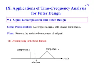
Applications on Time-Frequency Analysis Signal Decomposition and Filter Design A signal has several components -> separable in time -> separable in freq. -> separable in time-freq. f t t f 41

Applications on Time-Frequency Analysis Signal Decomposition and Filter Design An example f 1 0t t 1t 2 Rotation -> filtering in the FRFT domain 42

Applications on Time-Frequency Analysis Signal Decomposition and Filter Design An example [1] 43

Applications on Time-Frequency Analysis Signal Decomposition and Filter Design An example 2 2 2 + = + + 0.23 0.3 8.5 0.46 9.6 j t j t j t j t j t ( ) 0.5 0.5 0.5 n t e e e [1] 44

Applications on Time-Frequency Analysis Signal Decomposition and Filter Design An example 2 2 2 + = + + 0.23 0.3 8.5 0.46 9.6 j t j t j t j t j t ( ) 0.5 0.5 0.5 n t e e e [1] 45

Applications on Time-Frequency Analysis Signal Decomposition and Filter Design An example [1] 46

Applications on Time-Frequency Analysis Sampling Theory Nyquist theorem : , B Adaptive sampling 2 sf B [1] 47

Conclusions and Future work Comparison among STFT,GT,WDF rec-STFT GT WDF Complexity Clarity Time-frequency analysis apply to image processing? 48

References [1] Jian-Jiun Ding, Time frequency analysis and wavelet transform class note, the Department of Electrical Engineering, National Taiwan University (NTU), Taipei, Taiwan, 2007. [2] S. C. Pei and J. J. Ding, Relations between Gabor transforms and fractional Fourier transforms and their applications for signal processing , IEEE Trans. Signal Processing, vol.55,no. 10,pp.4839-4850. [3] S. Qianand D. Chen, Joint Time-Frequency Analysis: Methods and Applications, Prentice-Hall, 1996. [4] D. Gabor, Theory of communication , J. Inst. Elec. Eng., vol. 93, pp.429-457, Nov. 1946. [5] L. B. Almeida, The fractional Fourier transform and time-frequency representations, IEEE Trans. Signal Processing, vol. 42,no. 11, pp. 3084- 3091, Nov. 1994. [6] K. B. Wolf, Integral Transforms in Science and Engineering, Ch. 9: Canonical transforms, New York, Plenum Press, 1979. 49

References [7] X. G. Xia, On bandlimited signals with fractional Fourier transform, IEEE Signal Processing Letters, vol. 3, no. 3, pp. 72-74, March 1996. [8] L. Cohen, Time-Frequency Analysis, Prentice-Hall, New York, 1995. [9] T. A. C. M. Classen and W. F. G. Mecklenbrauker, The Wigner distribution a tool for time-frequency signal analysis; Part I, Philips J. Res., vol. 35, pp. 217-250, 1980. 50