Epochwise Back Propagation Through Time for Recurrent Networks

E
p
o
c
h
w
i
s
e
B
a
c
k
P
r
o
p
a
g
a
t
i
o
n
T
h
r
o
u
g
h
T
i
m
e
•
Let the
data set used to train
a recurrent network
be partitioned
into
independent epochs
.
•
each epoch
representing a
temporal pattern
of interest.
•
n
o
:
the start time of an epoch and
•
n
1
:
its end time.
•
Given this epoch, we may define the
cost function
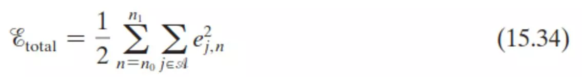
where
A
is the set of indices
j
pertaining to those neurons in
the network for which desired responses are specified,
e
j,n
is the error signal at the output
of such a neuron measured
with respect to some desired (target)
response.

•
We wish to compute sensitivity of the network, that
is, the
partial derivatives of the cost function
E
total
(n
o
,n
1
)
with
respect to the weights
of the
network.
•
To do so, we
may use the
epochwise BPTT
algorithm
,
which
builds on the batch mode
of
standard back-
propagation
learning
T
h
e
e
p
o
c
h
w
i
s
e
B
P
T
T
a
l
g
o
r
i
t
h
m
p
r
o
c
e
e
d
s
a
s
f
o
l
l
o
w
s
:
•
First,
a single forward pass
of the data through the network for the
interval (
n
o
,
n
1
) is performed, (The
complete record
of
input data
,
network state (i.e., synaptic
weights
of the network), and
desired
responses
over this interval
is
saved
).
•
A
single backward pass
over this past record is performed to
compute the values of the local gradients
where
’
(·) is the derivative of an activation function with respect
to its argument and v
j,n
is the induced local field of neuron
j
.
•
It is assumed that all neurons in the network have the same activation
function
(·).
•
The use of Eq. (15.36) is repeated, starting from time
n
1
and working back,
step by step
, to time
n
o
•
The number of
steps
involved here is equal to the number of
time-steps
contained in the epoch.
•
Once the computation of back propagation has been performed back to
time
n
o
+ 1, an
adjustment is applied to the synaptic weight w
ji
of neuron
j
,
given by
where
is the learning-rate parameter and
x
i
,
n
-1
is the input
applied to the
i
th synapse of neuron
j
at time
n
-1.
T
r
u
n
c
a
t
e
d
B
a
c
k
P
r
o
p
a
g
a
t
i
o
n
T
h
r
o
u
g
h
T
i
m
e
•
In BPTT the adjustments to the weights are made on a
continuous basis while the network is running.
•
In order to do this in a computationally feasible manner, we
save
the relevant
history of input data and network state
only
for a fixed number of time-steps
, called the
truncation depth
denoted by
h
.
•
Any
information older than
h
time-steps into the past is
considered irrelevant and may therefore be
ignored.
•
This form of the algorithm is called the “
truncated back-
propagation-through time BPTT(h) algorithm
”
•
The
local gradient
for neuron
j
is now defined by
T
r
u
n
c
a
t
e
d
B
a
c
k
P
r
o
p
a
g
a
t
i
o
n
T
h
r
o
u
g
h
T
i
m
e
In comparing Eq. (15.39) with (15.36), we see that, unlike the
epochwise BPTT algorithm, the
error signal
is injected into the
computation
only at the current time
n
.
1
5
.
8
R
E
A
L
-
T
I
M
E
R
E
C
U
R
R
E
N
T
L
E
A
R
N
I
N
G
(
R
T
R
L
)
•
The algorithm
derives its name
from the fact
that
adjustments are made
to the synaptic weights
of a fully
connected recurrent network
in real time
—that is, while the
network continues to perform its signal-processing function.
•
Figure 15.10 shows the layout of such a recurrent network.
•
It consists of
q
neurons
with
m
external inputs
.
•
The network has
two distinct layers
: a
concatenated input-
feedback
layer
and a
processing
layer of computation nodes
.
•
Correspondingly, the
synaptic connections
of the network
are
made up of
feedforward and feedback connections
FIGURE 15.10
Fully connected
recurrent network
for formulation of
the RTRL
algorithm
Input/feedback layer
Computation layer
1
5
.
8
R
E
A
L
-
T
I
M
E
R
E
C
U
R
R
E
N
T
L
E
A
R
N
I
N
G
3
•
The state-space description of the network is defined by Eqs.
(15.10) and (15.11), and is reproduced here in the expanded
form
where it is assumed that
all the neurons
have a
common
activation function
(·).
T
h
e
(
q
+
m
+
1
)
-
b
y
-
1
v
e
c
t
o
r
w
j
i
s
t
h
e
s
y
n
a
p
t
i
c
-
w
e
i
g
h
t
v
e
c
t
o
r
o
f
n
e
u
r
o
n
j
i
n
t
h
e
r
e
c
u
r
r
e
n
t
n
e
t
w
o
r
k
–
t
h
a
t
i
s
1
5
.
8
R
E
A
L
-
T
I
M
E
R
E
C
U
R
R
E
N
T
L
E
A
R
N
I
N
G
4
1
5
.
8
R
E
A
L
-
T
I
M
E
R
E
C
U
R
R
E
N
T
L
E
A
R
N
I
N
G
5
1
5
.
8
R
E
A
L
-
T
I
M
E
R
E
C
U
R
R
E
N
T
L
E
A
R
N
I
N
G
6
1
5
.
8
R
E
A
L
-
T
I
M
E
R
E
C
U
R
R
E
N
T
L
E
A
R
N
I
N
G
7
1
5
.
8
R
E
A
L
-
T
I
M
E
R
E
C
U
R
R
E
N
T
L
E
A
R
N
I
N
G
8
1
5
.
8
R
E
A
L
-
T
I
M
E
R
E
C
U
R
R
E
N
T
L
E
A
R
N
I
N
G
1
0
E
x
a
m
p
l
e
5
I
l
l
u
s
t
r
a
t
i
o
n
o
f
t
h
e
R
T
R
L
A
l
g
o
r
i
t
h
m
•
In this example, we formulate the RTRL algorithm for the fully
recurrent network shown in Fig. 15.6
•
with
two inputs
and a
single output
.
•
The network has
three neurons
, with the composition of
matrices
W
a
,
W
b
, and
W
c
as described in Example 1.
•
With
m
= 2,
q
= 3, and
p =
1, we find from Eq. (15.44) that
•
Where
kj
is the Kronecker delta, which is
equal to 1
for
k
=
j
and
zero otherwise
;
•
j, k = 1, 2, 3, and
l
= 1, 2, ..., 6.
•
Note that
W
a
={w
ji
},
for (j,i)= 1, 2, 3,
•
and
W
b
={w
jl
},
for
j
= 1, 2, 3 and
l
= 4, 5, 6.
Note that the index
at the
o/p is 1 because there is a
single o/p neuron
W
1
,
1
W
1
,
2
W
1
,
3
W
2
,
1
W
3
,
1
W
2
,
2
W
3
,
2
W
2
,
3
W
3
,
3
W
1
,
4
W
2
,
4
W
3
,
4
W
1
,
5
W
1
,
6
W
2
,
5
W
3
,
5
W
2
,
6
W
3
,
6
ب
ا
لا
م
ك
ا
ن
ا
س
ت
خ
د
ا
م
ا
ل
م
ص
د
ر
أ
د
ن
ا
ه
ل
غ
ر
ض
ت
و
ض
ي
ح
R
T
R
L
A
l
g
o
r
i
t
h
m
•
Dijk99-Recurrent-Neural-networks
•
pp63-64
In the context of training recurrent networks, Epochwise Back Propagation Through Time involves dividing the data set into independent epochs, each representing a specific temporal pattern of interest. The start time of each epoch, denoted by 'no', is crucial for capturing the sequential dependencies within the data. This approach enables the network to learn temporal relationships effectively by focusing on distinct patterns during each epoch, contributing to improved training performance in tasks such as sequence modeling and prediction.

Uploaded on Sep 21, 2024 | 0 Views
Download Presentation

Please find below an Image/Link to download the presentation.
The content on the website is provided AS IS for your information and personal use only. It may not be sold, licensed, or shared on other websites without obtaining consent from the author. Download presentation by click this link. If you encounter any issues during the download, it is possible that the publisher has removed the file from their server.
E N D
Presentation Transcript
Epochwise Back Propagation Through Time Epochwise Back Propagation Through Time Let the data set used to train a recurrent network be partitioned into independent epochs. each epoch representing a temporal pattern of interest. no :the start time of an epoch and n1 :its end time. Given this epoch, we may define the cost function where A is the set of indices j pertaining to those neurons in the network for which desired responses are specified, ej,n is the error signal at the output of such a neuron measured with respect to some desired (target) response.
We wish to compute sensitivity of the network, that is, the partial derivatives of the cost function Etotal(no,n1) with respect to the weights of the network. To do so, we may use the epochwise BPTT algorithm, which builds on the batch mode of standard back- propagation learning
The epochwise BPTT algorithm proceeds as follows: The epochwise BPTT algorithm proceeds as follows: First, a single forward pass of the data through the network for the interval (no, n1) is performed, (The complete record of input data, network state (i.e., synaptic weights of the network), and desired responses over this interval is saved). A single backward pass over this past record is performed to compute the values of the local gradients where ( ) is the derivative of an activation function with respect to its argument and vj,nis the induced local field of neuron j.
It is assumed that all neurons in the network have the same activation function ( ). The use of Eq. (15.36) is repeated, starting from time n1 and working back, step by step, to time no The number of steps involved here is equal to the number of time-steps contained in the epoch. Once the computation of back propagation has been performed back to time no+ 1, an adjustment is applied to the synaptic weight wjiof neuron j, given by where is the learning-rate parameter and xi, n-1 is the input applied to the ith synapse of neuron j at time n-1.
Truncated Back Propagation Through Time Truncated Back Propagation Through Time In BPTT the adjustments to the weights are made on a continuous basis while the network is running. In order to do this in a computationally feasible manner, we save the relevant history of input data and network state only for a fixed number of time-steps, called the truncation depth denoted by h. Any information older than h time-steps into the past is considered irrelevant and may therefore be ignored. This form of the algorithm is called the truncated back- propagation-through time BPTT(h) algorithm
Truncated Back Propagation Through Time Truncated Back Propagation Through Time The local gradient for neuron j is now defined by In comparing Eq. (15.39) with (15.36), we see that, unlike the epochwise BPTT algorithm, the error signal is injected into the computation only at the current time n.
15.8 15.8 REAL REAL- -TIME RECURRENT LEARNING (RTRL) TIME RECURRENT LEARNING (RTRL) The algorithm derives its name from the fact that adjustments are made to the synaptic weights of a fully connected recurrent network in real time that is, while the network continues to perform its signal-processing function. Figure 15.10 shows the layout of such a recurrent network. It consists of q neurons with m external inputs. The network has two distinct layers: a concatenated input- feedback layer and a processing layer of computation nodes. Correspondingly, the synaptic connections of the network are made up of feedforward and feedback connections
FIGURE 15.10 Fully connected recurrent network for formulation of the RTRL algorithm Input/feedback layer Computation layer
15.8 15.8 REAL REAL- -TIME RECURRENT LEARNING TIME RECURRENT LEARNING3 3 The state-space description of the network is defined by Eqs. (15.10) and (15.11), and is reproduced here in the expanded form where it is assumed that all the neurons have a common activation function ( ). The (q + m + 1)-by-1 vector wjis the synaptic-weight vector of neuron j in the recurrent network that is
15.8 15.8 REAL REAL- -TIME RECURRENT LEARNING TIME RECURRENT LEARNING4 4
15.8 15.8 REAL REAL- -TIME RECURRENT LEARNING TIME RECURRENT LEARNING5 5
15.8 15.8 REAL REAL- -TIME RECURRENT LEARNING TIME RECURRENT LEARNING6 6
15.8 15.8 REAL REAL- -TIME RECURRENT LEARNING TIME RECURRENT LEARNING7 7
15.8 15.8 REAL REAL- -TIME RECURRENT LEARNING TIME RECURRENT LEARNING8 8
15.8 15.8 REAL REAL- -TIME RECURRENT LEARNING TIME RECURRENT LEARNING10 10
Example Example 5 5 Illustration of the RTRL Algorithm Illustration of the RTRL Algorithm In this example, we formulate the RTRL algorithm for the fully recurrent network shown in Fig. 15.6 with two inputs and a single output. The network has three neurons, with the composition of matrices Wa, Wb, and Wc as described in Example 1. With m = 2, q = 3, and p = 1, we find from Eq. (15.44) that
Wc= (1, 0, 0) Note that the indexat the o/p is 1 because there is a single o/p neuron Where kjis the Kronecker delta, which is equal to 1 for k = j and zero otherwise; j, k = 1, 2, 3, and l = 1, 2, ..., 6. Note that Wa={wji}, for (j,i)= 1, 2, 3, and Wb={wjl}, for j = 1, 2, 3 and l = 4, 5, 6.
W1,1 W3,1 W2,1 W1,2 W2,2 W3,2 W1,3 W2,3 W3,3 W1,4 W2,4 W3,4 W1,5 W2,5 W3,5 W2,6 W1,6 W3,6