Electric Flux and Analogies in Electromagnetism
Prof. David R. Jackson
Dept. of ECE
S
p
r
i
n
g
2
0
2
4
Notes 9
Flux
ECE 3318
ECE 3318
Applied Electricity and Magnetism
Applied Electricity and Magnetism
1
Notes prepared by the EM Group
University of Houston
Flux Density
Flux Density
D
e
f
i
n
e
:
“flux density vector”
2
From Coulomb’s law:
We then have
Charge in free space
Flux lines
(Flux lines show us the direction of the electric field vector.)
(This definition holds in free space.)
Flux Through Surface
Flux Through Surface
Define flux through a surface:
3
N
o
t
e
:
In this picture, flux is the flux crossing the
surface in the
outward
sense.
Cross-sectional view
Charge in free space
Example
Example
(We want the flux going out.)
Find the flux from a point charge
going
out
through a spherical surface.
4
Example (cont.)
Example (cont.)
5
Current Analogy
Current Analogy
6
Analogy with electric current
A small electrode in a conducting
medium spews out current equally
in all directions.
Cross-sectional view
Conducting medium
7
Current Analogy (cont.)
Current Analogy (cont.)
Free-space
Conducting medium
Electric Flux
Current
Water Analogy
Water Analogy
8
Each electric flux line is
like a stream of water.
F
n
=
flow rate of water out of nozzle [
m
3
/s
]
Each stream of water carries
F
n
/
N
[
m
3
/s
].
Note that the flow rate through a closed surface is
F
s
=
F
n
.
F
s
=
flow rate of water out of surface [
m
3
/s
]
Water Analogy (cont.)
Water Analogy (cont.)
9
Here is a real “flux fountain”
(Wortham fountain, a.k.a. the “Dandelion” on Allen Parkway).
10
Analogy example:
Find
F
s
(flow rate through surface
S
)
Water Analogy (cont.)
Water Analogy (cont.)
Flux through a Surface using Flux Lines
Flux through a Surface using Flux Lines
(Point Charge)
(Point Charge)
11
E
x
a
m
p
l
e
:
Find
(flux through surface
S
)
Flux in 2-D Problems
Flux in 2-D Problems
We now define the
flux per meter
in the
z
direction.
12
We can think of
l
as being
the flux
through a surface
S
that is the contour
C
extruded
one meter
in the
z
direction.
2
-
D
p
r
o
b
l
e
m
s
:
E
v
e
r
y
t
h
i
n
g
i
s
i
n
f
i
n
i
t
e
a
n
d
n
o
t
c
h
a
n
g
i
n
g
i
n
t
h
e
z
d
i
r
e
c
t
i
o
n
.
Line charge in free space
Flux Plot (2-D)
Flux Plot (2-D)
Rules for a 2-D flux plot:
13
Flux plot for a line charge
1)
Flux lines are in the direction of the electric field*.
2)
The magnitude of the electric field is inversely proportional to the spacing
between flux lines**.
3)
Flux lines come out of positive charges and end on negative charges (they
cannot stop or begin in free space)***.
*
A convention we adopt.
**
A convention we adopt.
*** A consequence of Gauss’s law.
Example
Example
Line charge
14
Notice how the flux lines get closer as we approach
the line charge: there is a stronger electric field there.
According to rule #2:
If
W
is the distance between flux lines:
This happens automatically in this
example by choosing a fixed number of
equally-spaced flux lines.
Flux Property in 2-D Flux Plots
Flux Property in 2-D Flux Plots
N
C
is defined as the number of flux lines through
C.
The flux (per meter)
l
through a contour is
proportional
to the
number of flux lines that cross the contour.
15
Please see the Appendix for a proof of this flux property.
N
o
t
e
:
The constant of proportionality depends on how
many flux lines you decide to draw.
Example
Example
Graphically evaluate
16
N
o
t
e
:
The answer will be more accurate if we
use a plot with more flux lines!
G
o
a
l
:
L
i
n
e
c
h
a
r
g
e
e
x
a
m
p
l
e
17
Equipotential Contours
Equipotential Contours
An equipotential contour
C
V
is a contour on which the
potential is constant
.
Equipotential Contours (cont.)
Equipotential Contours (cont.)
18
Property:
The flux line are always perpendicular
to the equipotential contours.
(proof on next slide)
Equipotential Contours (cont.)
Equipotential Contours (cont.)
Proof:
On
C
V
:
19
C
o
n
c
l
u
s
i
o
n
:
T
h
e
r
v
e
c
t
o
r
(
l
y
i
n
g
o
n
C
V
)
i
s
p
e
r
p
e
n
d
i
c
u
l
a
r
t
o
t
h
e
f
l
u
x
l
i
n
e
s
.
Two nearby points on an equipotential
contour are considered.
P
r
o
o
f
o
f
p
e
r
p
e
n
d
i
c
u
l
a
r
p
r
o
p
e
r
t
y
:
Method of Curvilinear Squares
Method of Curvilinear Squares
Assume a
constant voltage difference
V
between adjacent equipotential lines
in a 2-D flux plot.
2-D Flux Plot
N
o
t
e
:
Along a flux line, the voltage always
decreases
as
we go in the direction of the flux line.
20
N
o
t
e
:
It is called a curvilinear “square” even though the
shape may be rectangular.
A
s
s
u
m
p
t
i
o
n
:
Method of Curvilinear Squares (cont.)
Method of Curvilinear Squares (cont.)
T
h
e
o
r
e
m
:
T
h
e
s
h
a
p
e
(
a
s
p
e
c
t
r
a
t
i
o
L
/
W
)
o
f
t
h
e
“
c
u
r
v
i
l
i
n
e
a
r
s
q
u
a
r
e
s
”
i
s
p
r
e
s
e
r
v
e
d
t
h
r
o
u
g
h
o
u
t
t
h
e
f
l
u
x
p
l
o
t
.
21
Assumption:
V
is constant throughout plot.
Proof
of constant aspect ratio property
If we integrate along the flux line,
E
is in the same direction as
d
r
.
so
Therefore
Method of Curvilinear Squares (cont.)
Method of Curvilinear Squares (cont.)
Hence,
22
Also,
Hence,
so
Method of Curvilinear Squares (cont.)
Method of Curvilinear Squares (cont.)
23
Hence,
(proof complete)
R
e
m
i
n
d
e
r
:
In a flux plot the magnitude of
the electric field is
inversely
proportional
to the spacing
between the flux lines.
The constant
C
1
is some constant of proportionality.
Example
Example
Line charge
The aspect ratio
L
/
W
has been chosen to be
unity
in this plot.
In this example
L
and
W
are both proportional to the radius
.
24
Notice how the flux lines get
closer as we approach the line
charge: there is a stronger
electric field there.
Example
Example
25
A parallel-plate capacitor
Note:
L
/
W
0.5
Example
Example
Figure 6-8 in the Hayt and Buck book (9
th
Ed.).
Coaxial cable with a square inner conductor
26
Making a Flux Plot
Making a Flux Plot
27
Rule 1: We start with
equipotential contours having
a fixed
V
between.
Rule 2: Flux lines are drawn perpendicular to the equipotential contours.
Rule 3:
L
/
W
is kept constant throughout the plot.
I
f
a
l
l
t
h
e
s
e
r
u
l
e
s
a
r
e
f
o
l
l
o
w
e
d
,
t
h
e
n
w
e
h
a
v
e
t
h
e
f
o
l
l
o
w
i
n
g
p
r
o
p
e
r
t
i
e
s
:
Flux lines are in direction of
E
.
The magnitude of the electric field is inversely proportional to
the spacing between the flux lines.
Here are the rules for making a 2-D flux plot, assuming that we start
with equipotential contours separated by a fixed value of
V
*:
* This is what you will be doing in the class project.
Example
Example
28
In the class project, you will be drawing in flux lines.
Parallel-plate capacitor region
(The equipotential contours come from Excel.)
Example (cont.)
Example (cont.)
29
30
http://en.wikipedia.org/wiki/Electrostatics
Flux lines are closer
together where the field is
stronger.
The field is strong near a
sharp conducting corner.
Flux lines begin on positive
charges and end on
negative charges.
Flux lines enter a conductor
perpendicular to it.
S
o
m
e
o
b
s
e
r
v
a
t
i
o
n
s
:
Flux Plot with Conductors
Flux Plot with Conductors
Conductor
Example of Electric Flux Plot
Example of Electric Flux Plot
31
E
l
e
c
t
r
o
p
o
r
a
t
i
o
n
-
m
e
d
i
a
t
e
d
t
o
p
i
c
a
l
d
e
l
i
v
e
r
y
o
f
v
i
t
a
m
i
n
C
f
o
r
c
o
s
m
e
t
i
c
a
p
p
l
i
c
a
t
i
o
n
s
Lei Zhang
a,
, Sheldon Lerner
b
, William V Rustrum
a
, Günter A Hofmann
a
a
Genetronics Inc., 11199 Sorrento Valley Rd., San Diego, CA 92121, USA
b
Research Institute for Plastic, Cosmetic and Reconstructive Surgery Inc., 3399 First Ave., San
Diego, CA 92103, USA.
N
o
t
e
:
In this example, the
aspect ratio
L
/
W
is not
held constant
!
Example of Magnetic Flux Plot
Example of Magnetic Flux Plot
Solenoid wrapped around a ferrite core (cross sectional view)
Flux plots are often
used to display the
results of a numerical
simulation, for either
the electric field or the
magnetic field.
32
Magnetic flux lines
Ferrite core
Solenoid windings
Appendix:
Appendix:
Proof of Flux Property
Proof of Flux Property
33
Proof of Flux Property
Proof of Flux Property
N
C
: flux lines
Through
C
so
or
34
One small piece of the contour
(the length is
L
)
Flux Property Proof (cont.)
Flux Property Proof (cont.)
Also,
(from the property of a flux plot)
Hence, substituting into the above equation, we have
Therefore,
35
(proof complete)
Concept of electric flux, flux density, and surface flux in electromagnetism. Learn how to calculate flux through surfaces and understand the water analogy to visualize flux lines. Analogies with electric current and conducting mediums are also discussed. Delve into examples and analogies to deepen your understanding of these fundamental electromagnetic concepts.

Download Presentation

Please find below an Image/Link to download the presentation.
The content on the website is provided AS IS for your information and personal use only. It may not be sold, licensed, or shared on other websites without obtaining consent from the author.If you encounter any issues during the download, it is possible that the publisher has removed the file from their server.
You are allowed to download the files provided on this website for personal or commercial use, subject to the condition that they are used lawfully. All files are the property of their respective owners.
The content on the website is provided AS IS for your information and personal use only. It may not be sold, licensed, or shared on other websites without obtaining consent from the author.
E N D
Presentation Transcript
ECE 3318 Applied Electricity and Magnetism Spring 2024 Prof. David R. Jackson Dept. of ECE Notes 9 Flux Notes prepared by the EM Group University of Houston 1
Flux Density q From Coulomb s law: = r E 2 4 r 0 12 8.854187818 10 F/m E 0 Flux lines (Flux lines show us the direction of the electric field vector.) q Define: D E flux density vector 0 Charge in free space (This definition holds in free space.) We then have q = 2 2 [C/m ] D r 4 r 2
Flux Through Surface Define flux through a surface: E C n D ndS S Note: In this picture, flux is the flux crossing the surface in the outward sense. q S q = 2 2 [C/m ] D r 4 r Cross-sectional view Charge in free space 3
Example z Find the flux from a point charge going out through a spherical surface. n D D ndS r S q y = D r dS S S x q = r r dS 2 4 q r S = + n r = dS (We want the flux going out.) 2 4 r S 4
Example (cont.) 2 q = d d 2 sin r 2 4 r 0 0 q 2 = d d sin 4 0 0 2 q = sin d d 4 0 0 q ( )( ) 2 = 2 4 = [ ] q C 5
Current Analogy Conducting medium Analogy with electric current n A = J ndS I S A small electrode in a conducting medium spews out current equally in all directions. I S J I = 2 2 A/m J r 4 r Cross-sectional view 6
Current Analogy (cont.) Current Electric Flux J D Conducting medium Free-space I q I q = 2 2 [A/m ] J r = 2 2 [C/m ] D r 4 r 4 r C A D ndS = J ndS I S S 7
Water Analogy z Each electric flux line is like a stream of water. N streamlines Water streams Each stream of water carries Fn / N [m3/s]. S n F y x Water nozzle (omnidirectional) Fn =flow rate of water out of nozzle [m3/s] Fs =flow rate of water out of surface [m3/s] Note that the flow rate through a closed surface is Fs =Fn. 8
Water Analogy (cont.) Here is a real flux fountain (Wortham fountain, a.k.a. the Dandelion on Allen Parkway). 9
Water Analogy (cont.) Analogy example: ( ) = 3 15 m /s n F flow rate from central node ( ) N = 1000 number of pipes S ( ) N = 20 number of flux lines through surface S s Find Fs (flow rate through surface S) 3 15 m /s 1000 pipes ( ) 0.3 m /s = = 3 20pipes sF 10
Flux through a Surface using Flux Lines (Point Charge) z Example: E q = 15 C ( ) q N = 1000 number of flux lines y ( ) S N = 20 number of flux lines through surface S s Find (flux through surface S) x 15 C ( ) = = 20flux lines 0.3 C 1000 flux lines 11
Flux in 2-D Problems 2-D problems: Everything is infinite and not changing in the z direction. We now define the flux per meter in the z direction. E n D ndl C/m l C We can think of las being the flux through a surface S that is the contour C extruded one meter in the z direction. 0 l C 0 l Line charge in free space C = D ndS S 1 m S ( ) 1 m = = l l C 12
Flux Plot (2-D) Rules for a 2-D flux plot: 1) Flux lines are in the direction of the electric field*. 2) The magnitude of the electric field is inversely proportional to the spacing between flux lines**. 3) Flux lines come out of positive charges and end on negative charges (they cannot stop or begin in free space)***. y Flux plot for a line charge = * A convention we adopt. **A convention we adopt. *** A consequence of Gauss s law. 0 l E 2 0 x 0 l 13
Example Line charge Notice how the flux lines get closer as we approach the line charge: there is a stronger electric field there. l 0C/m y = 0 l E 2 0 According to rule #2: If W is the distance between flux lines: W x W This happens automatically in this example by choosing a fixed number of equally-spaced flux lines. 14
Flux Property in 2-D Flux Plots The flux (per meter) lthrough a contour is proportional to the number of flux lines that cross the contour. NC is defined as the number of flux lines through C. E n D ndl N l C C C Note: The constant of proportionality depends on how many flux lines you decide to draw. General E field Please see the Appendix for a proof of this flux property. 15
Example y l = 1 C/m 0 Goal: N = Choose: 16 f Graphically evaluate = D ndl C l C x 1 C/m 16 lines ( ) = 4 lines l 1 4 Note: = C/m The answer will be more accurate if we use a plot with more flux lines! l 16
Equipotential Contours An equipotential contour CV is a contour on which the potential is constant. y Line charge example E Flux lines 0 l x = 1 V Equipotential contours CV = 0 V = + 1 V 17
Equipotential Contours (cont.) Property: E C V The flux line are always perpendicular to the equipotential contours. C E V (proof on next slide) ( = constant ) 18
Equipotential Contours (cont.) Proof of perpendicular property: Proof: Two nearby points on an equipotential contour are considered. On CV : B = E dr V = 0 AB A B E dr C = 0 E r V A E = E r B E r r A Conclusion: The r vector (lying on CV) is perpendicular to the flux lines. 19
Method of Curvilinear Squares 2-D Flux Plot C V E V + Assumption: B Assume a constant voltage difference Vbetween adjacent equipotential lines in a 2-D flux plot. A Note: Along a flux line, the voltage always decreases as we go in the direction of the flux line. Curvilinear square Note: It is called a curvilinear square even though the shape may be rectangular. 20
Method of Curvilinear Squares (cont.) Theorem: The shape (aspect ratio L/W) of the curvilinear squares is preserved throughout the flux plot. Assumption: V is constant throughout plot. C V E + V E C V W L + V L W =constant 21
Method of Curvilinear Squares (cont.) Proof of constant aspect ratio property C B V E V = E dr = V V + AB A dr W B = dl dr L A If we integrate along the flux line, E is in the same direction as dr . E dr E dr = ( ) = o cos 0 E dl B = = V E dl V Hence, AB A B E dl V E L V so Therefore A 22
Method of Curvilinear Squares (cont.) Hence, V E = L C + V V E W Also, B L 1 Reminder: A E In a flux plot the magnitude of the electric field is inversely proportional to the spacing between the flux lines. W so 1 E = W C The constant C1 is some constant of proportionality. 1 Hence, 1 C L W = = V constant (proof complete) 1 23
Example Line charge y Notice how the flux lines get closer as we approach the line charge: there is a stronger electric field there. l 0C/m 1 1 E W x L W The aspect ratio L/W has been chosen to be unity in this plot. In this example L and W are both proportional to the radius . 24
Example A parallel-plate capacitor Note:L / W 0.5 25
Example Coaxial cable with a square inner conductor L W = 1 Figure 6-8 in the Hayt and Buck book (9th Ed.). 26
Making a Flux Plot Here are the rules for making a 2-D flux plot, assuming that we start with equipotential contours separated by a fixed value of V*: Rule 1: We start with equipotential contours having a fixed V between. Rule 2: Flux lines are drawn perpendicular to the equipotential contours. Rule 3: L / Wis kept constant throughout the plot. If all these rules are followed, then we have the following properties: Flux lines are in direction of E. The magnitude of the electric field is inversely proportional to the spacing between the flux lines. * This is what you will be doing in the class project. 27
Example In the class project, you will be drawing in flux lines. (The equipotential contours come from Excel.) 1 6 1 1 2 2 3 3 4 4 5 5 6 6 7 7 8 8 9 9 1 1 1 1 0-0.2 0.2 0.2-0.4 0.4 0.4-0.6 0.6 0.6-0.8 0.8 0.8-1 1.0 V 0 V Contour Plot Task 2 Parallel-plate capacitor region 28
Example (cont.) In the class project, you will be drawing in flux lines. 1 6 1 1 2 2 3 3 4 4 5 5 6 6 7 7 8 8 9 9 1 1 1 1 0-0.2 0.2-0.4 0.4-0.6 0.6-0.8 0.8-1 Contour Plot Task 2 Parallel-plate capacitor region 29
Flux Plot with Conductors Conductor Some observations: Flux lines are closer together where the field is stronger. The field is strong near a sharp conducting corner. Flux lines begin on positive charges and end on negative charges. Flux lines enter a conductor perpendicular to it. http://en.wikipedia.org/wiki/Electrostatics 30
Example of Electric Flux Plot Note: In this example, the aspect ratio L/W is not held constant! Electroporation-mediated topical delivery of vitamin C for cosmetic applications Lei Zhanga, , Sheldon Lernerb, William V Rustruma, G nter A Hofmanna a Genetronics Inc., 11199 Sorrento Valley Rd., San Diego, CA 92121, USA b Research Institute for Plastic, Cosmetic and Reconstructive Surgery Inc., 3399 First Ave., San Diego, CA 92103, USA. 31
Example of Magnetic Flux Plot Solenoid wrapped around a ferrite core (cross sectional view) Flux plots are often used to display the results of a numerical simulation, for either the electric field or the magnetic field. Magnetic flux lines Solenoid windings Ferrite core 32
Appendix: Proof of Flux Property 33
Proof of Flux Property E L NC: flux lines Through C E C n L C One small piece of the contour (the length is L) C =number of flux lines N C ( ) D n = cos L D L E l L ( ) cos D L so l L ( ) D L or l 34
Flux Property Proof (cont.) ( ) D L l E Also, L N 1/ D L C (from the property of a flux plot) Hence, substituting into the above equation, we have N L ( ) = C D L L N l C N Therefore, (proof complete) l C 35


")

")

")
")


")


")
")

")
")
")


")


")