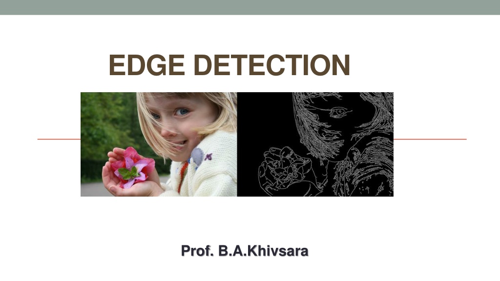
EDGE DETECTION
E
D
G
E
D
E
T
E
C
T
I
O
N
P
P
r
r
o
o
f
f
.
.
B
B
.
.
A
A
.
.
K
K
h
h
i
i
v
v
s
s
a
a
r
r
a
a
What is Edge Detection?
•
Identifying points/Edges in a digital image at which the image
brightness changes sharply or has discontinuities.
•
- Edges are significant local changes of intensity in an image.
•
- Edges typically occur on the boundary between two different regions in an
image.
G
o
a
l
o
f
e
d
g
e
d
e
t
e
c
t
i
o
n
TYPES OF EDGES
Process of Edge Detection
P
r
o
c
e
s
s
o
f
E
d
g
e
D
e
t
e
c
t
i
o
n
-
N
N
o
o
i
i
s
s
e
e
r
r
e
e
d
d
u
u
c
c
t
t
i
i
o
o
n
n
O
r
i
g
i
n
a
l
I
m
a
g
e
A
f
t
e
r
N
o
i
s
R
e
d
u
c
t
i
o
n
P
r
o
c
e
s
s
o
f
E
d
g
e
D
e
t
e
c
t
i
o
n
-
E
d
g
e
e
n
h
a
n
c
e
m
e
n
t
METHODS OF EDGE DETECTION
First
Order
Derivative
Gradient
•
For a continuous two dimensional function Gradient is defined as
Gradient Methods – Roberts Operator
Roberts Operator - Example
Gradient Methods – Sobel Operator
G
x
=
G
y
=
Sobel Operator - Example
Outputs of Sobel (top) and Roberts
operator
Second Order Derivative Methods
Second Order Derivative Methods - Laplacian
•
Defined as
•
Mask
•
Very susceptible to noise, filtering required, use Laplacian of
Gaussian
S
e
c
o
n
d
O
r
d
e
r
D
e
r
i
v
a
t
i
v
e
M
e
t
h
o
d
s
-
L
a
p
l
a
c
i
a
n
o
f
G
a
u
s
s
i
a
n
Program
•
#Libraries to be installed
# sudo apt-get install python-opencv
# sudo apt-get install python-matplotlib
import cv2
from matplotlib import pyplot as plt
img0 = cv2.imread('images.jpeg',)# loading imagegray = cv2.cvtColor(img0, cv2.COLOR_BGR2GRAY)# converting to gray scale
img = cv2.GaussianBlur(gray,(3,3),0)
•
# remove noise cv2.GaussianBlur(image,(Kernal_Hieght,Kernal_Width),SigmaX)
Program
•
# convolute with proper kernels
laplacian = cv2.Laplacian(img,cv2.CV_64F)
sobelx = cv2.Sobel(img,cv2.CV_64F,1,0) # x
sobely = cv2.Sobel(img,cv2.CV_64F,0,1) # y
•
plt.subplot(2,2,1),plt.imshow(img,cmap = 'gray')
plt.title('Original'), plt.xticks([]), plt.yticks([])plt.subplot(2,2,2),plt.imshow(laplacian,cmap = 'gray')
plt.title('Laplacian'), plt.xticks([]), plt.yticks([])plt.subplot(2,2,3),plt.imshow(sobelx,cmap = 'gray')
plt.title('Sobel X'), plt.xticks([]), plt.yticks([])plt.subplot(2,2,4),plt.imshow(sobely,cmap = 'gray')
plt.title('Sobel Y'), plt.xticks([]), plt.yticks([])plt.show()
Edge detection is a crucial process in image analysis to identify points where image brightness changes sharply or has discontinuities, typically occurring at boundaries between different regions. This technique is extensively used for image segmentation and object extraction, involving steps like noise reduction and edge enhancement. Various methods like First Order Derivative, Second Order Derivative, and Canny Edge Detection are employed to achieve accurate edge detection in digital images.

Download Presentation

Please find below an Image/Link to download the presentation.
The content on the website is provided AS IS for your information and personal use only. It may not be sold, licensed, or shared on other websites without obtaining consent from the author.If you encounter any issues during the download, it is possible that the publisher has removed the file from their server.
You are allowed to download the files provided on this website for personal or commercial use, subject to the condition that they are used lawfully. All files are the property of their respective owners.
The content on the website is provided AS IS for your information and personal use only. It may not be sold, licensed, or shared on other websites without obtaining consent from the author.
E N D
Presentation Transcript
EDGE DETECTION Prof. B.A.Khivsara
What is Edge Detection? Identifying points/Edges in a digital image at which the image brightness changes sharply or has discontinuities. - Edges are significant local changes of intensity in an image. - Edges typically occur on the boundary between two different regions in an image.
Goal of edge detection Edge detection is extensively used in image segmentation when we want to divide the image into areas corresponding to different objects. If we need to extract different object from an image, we need Edge Detection. Using Edge Detection, we can- recognition, Image comparizon, Unaccepted object can be remove.
TYPES OF EDGES Variation of Intensity / Gray Level Step Edge Ramp Edge Line Edge Roof Edge
Process of Edge Detection There are three steps to perform edge detection: Noise reduction Edge Detection Identify edges enhancement
Process of Edge Detection - Noise reduction where we try to suppress as much noise as possible, without smoothing away the meaningful edges. Original Image After Nois Reduction
Process of Edge Detection - Edge enhancement where we apply some kind of filter that responds strongly at edges and weakly elsewhere.
METHODS OF EDGE DETECTION First Order Derivative / Gradient Methods Roberts Operator Sobel Operator Prewitt Operator Second Order Derivative Laplacian Laplacian of Gaussian Optimal Edge Detection Canny Edge Detection
First Order Derivative At the point of greatest slope, the first derivative has maximum value E.g. For a Continuous 1- dimensional function f(t)
Gradient For a continuous two dimensional function Gradient is defined as f Gx x = = [ ( , )] G f x y f Gy y = + + 2 2 G Gx Gy Gx Gy Gy = 1 tan Gx
Gradient Methods Roberts Operator Convolution Mask 0 -1 1 0 Gx = 0 1 -1 0 Gy=
Roberts Operator - Example The output image has been scaled by a factor of 5 Spurious dots indicate that the operator is susceptible to noise
Gradient Methods Sobel Operator The 3X3 convolution mask smoothes the image by some amount , hence it is less susceptible to noise. But it produces thicker edges. So edge localization is poor Convolution Mask 1 0 -1 2 0 -2 1 0 -1 -1 -2 -1 0 0 0 1 2 1 Gx= Gy=
Sobel Operator - Example Compare the output of the Sobel Operator with Roberts The spurious edges are still present but they are relatively less intense Roberts operator has missed a few edges Sobel operator detects thicker edges Outputs of Sobel (top) and Roberts operator
Second Order Derivative Methods Zero crossing of the second derivative of a function indicates the presence of a maxima
Second Order Derivative Methods - Laplacian Defined as Mask 0 1 0 1 -4 1 0 1 0 Very susceptible to noise, filtering required, use Laplacian of Gaussian
Second Order Derivative Methods - Laplacian of Gaussian Steps Smooth the image using Gaussian filter Enhance the edges using Laplacian operator Zero crossings denote the edge location Use linear interpolation to determine the sub-pixel location of the edge
Program #Libraries to be installed # sudo apt-get install python-opencv # sudo apt-get install python-matplotlib import cv2 from matplotlib import pyplot as plt img0 = cv2.imread('images.jpeg',)# loading image gray = cv2.cvtColor(img0, cv2.COLOR_BGR2GRAY)# converting to gray scale img = cv2.GaussianBlur(gray,(3,3),0) # remove noise cv2.GaussianBlur(image,(Kernal_Hieght,Kernal_Width),SigmaX)
Program # convolute with proper kernels laplacian = cv2.Laplacian(img,cv2.CV_64F) sobelx = cv2.Sobel(img,cv2.CV_64F,1,0) # x sobely = cv2.Sobel(img,cv2.CV_64F,0,1) # y plt.subplot(2,2,1),plt.imshow(img,cmap = 'gray') plt.title('Original'), plt.xticks([]), plt.yticks([]) plt.subplot(2,2,2),plt.imshow(laplacian,cmap = 'gray') plt.title('Laplacian'), plt.xticks([]), plt.yticks([]) plt.subplot(2,2,3),plt.imshow(sobelx,cmap = 'gray') plt.title('Sobel X'), plt.xticks([]), plt.yticks([]) plt.subplot(2,2,4),plt.imshow(sobely,cmap = 'gray') plt.title('Sobel Y'), plt.xticks([]), plt.yticks([]) plt.show()