Differential Equations and Laplace Transforms in Signal Processing

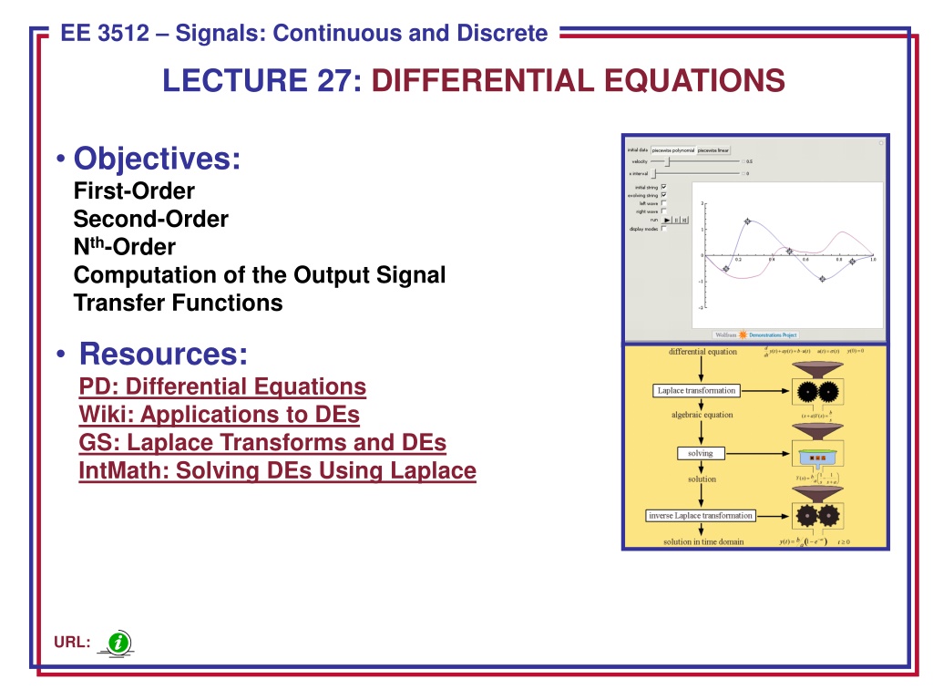
ECE 8443 Pattern Recognition EE 3512 Signals: Continuous and Discrete LECTURE 27: DIFFERENTIAL EQUATIONS Objectives: First-Order Second-Order Nth-Order Computation of the Output Signal Transfer Functions Resources: PD: Differential Equations Wiki: Applications to DEs GS: Laplace Transforms and DEs IntMath: Solving DEs Using Laplace URL:

First-Order Differential Equations Consider a linear time-invariant system defined by: ) ( t bx t ay dt dy t + = ( ) ( ) Apply the one-sided Laplace transform: + = ( ) 0 ( y ) ( ) ( ) sY s aY s bX s We can now use simple algebraic manipulations to find the solution: s bX y s Y a s + = + ) ( ) 0 ( ) ( ( ) ( ) 0 ( ) ( ) y bX s = + Y s + + s a s a If the initial condition is zero, we can find the transfer function: b s X + ) ( ( ) Y s = = ( ) H s s a Why is this transfer function, which ignores the initial condition, of interest? (Hints: stability, steady-state response) Note we can also find the frequency response of the system: b s H e H j s + = = j ( ) ( ) = j a How does this relate to the frequency response found using the Fourier transform? Under what assumptions is this expression valid? EE 3512: Lecture 27, Slide 1

RC Circuit The input/output differential equation: ( ) 1 1 dy t + = ( ) ( ) y t x t dt RC RC 0 ( y ) / 1 s RC = + ( ) ( ) Y s X s / 1 + / 1 + s RC RC Assume the input is a unit step function: 1 = = ( ) ( ) ( ) x t u t X s s 0 ( ) / 1 1 0 ( ) 1 1 y + RC / 1 + y + = + = + ( ) Y s / 1 + / 1 / 1 s RC s RC s s RC s s RC We can take the inverse Laplace transform to recover the output signal: 0 , 1 ) 0 ( ) ( + = t e e y t y / 1 ( / 1 ( ) ) RC t RC t For a zero initial condition: 1 ) ( = e t y / 1 ( ) RC t , 0 t Observations: How can we find the impulse response? Implications of stability on the transient response? What conclusions can we draw about the complete response to a sinusoid? EE 3512: Lecture 27, Slide 2

Second-Order Differential Equation Consider a linear time-invariant system defined by: ) ( ) ( 0 1 2 = + + t y a dt dt 2 ( ) d y t dy t dx t + = ( ) ( ) assume 0 ( x ) 0 a b b x t 1 0 dt Apply the Laplace transform: ( ) dy t + + = + 2 ( ) 0 ( y ) [ ( ) 0 ( y )] ( ) ( ) ( ) s Y s s a sY s a Y s b sX s b X s 1 0 1 0 dt = 0 t + + + 0 ( y ) 0 ( a + ) + 0 ( y ) b + s b + s y a = + 1 0 1 ( ) ( ) Y s X s 2 2 s s a s a s a 1 0 1 0 If the initial conditions are zero: ) ( ) ( s s X What is the nature of the impulse response of this system? + b + s b + Y s = = 1 0 H s 2 ( ) a s a How do the coefficients a0 and a1 influence the impulse response? 1 0 Example: y d 2 ( 2 ) ( ) 2 t dy t + + = = 6 8 ( ) 2 ( ) ( ) y t x t H s + + 2 dt 6 8 dt s s = / 1 = ( ) ( ) ( ) x t u t X s s 2 1 s . 0 25 s 5 . 0 + t . 0 s 25 + = = + ( ) Y s + + 2 2 4 s 6 8 e s s = 5 . 0 + 2 4 t t ( ) . 0 25 . 0 25 , 0 y t e EE 3512: Lecture 27, Slide 3

Nth-Order Case Consider a linear time-invariant system defined by: i N b dt dt + + + = ... 2 1 0 i 1 ( ) N = ( ) M ( ) d y t d y t d x t = + = ( ) a M N i i N i i dt 0 0 i i 2 M ... 2 b b + s b + s b + s 0 1 2 M ( ) H s N a a s a s s Example: + + 2 2 16 + 1 + s s = = ( ) ( ) H s X s + 3 2 2 s 4 8 s s s + s + s + 2 2 + 16 1 2 1 s 2 s s s = = = + + ( ) ( ) ( ) Y s H s X s ( )( ) + + + + + 3 2 2 s 4 8 2 ( ) 2 4 s s s 1 ( ) 2 ( ) 2 = + 2 2 t t ( ) cos sin 1 2 , 0 y t e t t e t 2 Could we have predicted the final value of the signal? Note that all circuits involving discrete lumped components (e.g., RLC) can be solved in terms of rational transfer functions. Further, since typical inputs are impulse functions, step functions, and periodic signals, the computations for the output signal always follows the approach described above. Transfer functions can be easily created in MATLAB using tf(num,den). EE 3512: Lecture 27, Slide 4

Circuit Analysis Voltage/Current Relationships: Diff. Eq. : Laplace Transform : = = ( ) ( ) ( ) ( ) v t Ri t V s RI s ( ) 1 C 1 1 s dv t = = + ( ) ( ) ( ) ) 0 ( v i t V s I s dt Cs = ( ) ( ) ( ) ) 0 ( Li di t V s LsI s = ( ) v t L dt Series Connections (Voltage Divider): ( ) Z s = 1 + ( ) ( ) V s V s 1 ( ) Z ( ) Z s Z s 1 2 ( ) s = 2 + ( ) ( ) V s V s 2 ( ) ( ) Z s Z s 1 2 EE 3512: Lecture 27, Slide 5

Circuit Analysis (Cont.) Parallel Connections (Current Divider): ( ) Z s = 2 + ( ) ( ) I s I s 1 ( ) Z ( ) Z s Z s 1 2 ( ) s = 1 + ( ) ( ) I s I s 2 ( ) ( ) Z s Z s 1 2 Example: / 1 R Cs = ( ) ( ) V s X s c + / 1 ( + ) Ls Cs ( ) V s / 1 LC = = c ( ) H s + / 1 ( + 2 ( ) X s ( / ) ) s R L s LC R = ( ) ( ) V s X s R + / 1 ( + ) Ls R Cs ( ) V s ( / ) R L s = = c ( ) H s + / 1 ( + 2 ( ) X s ( / ) ) s R L s LC Note the denominator of the transfer function did not change. Why? EE 3512: Lecture 27, Slide 6

RLC Circuit Consider computation of the transfer function relating the current in the capacitor to the input voltage. Strategy: convert the circuit to its Laplace transform representation, and use normal circuit analysis tools. Compute the voltage across the capacitor using a voltage divider, and then compute the current through the capacitor. Alternately, can use KVL, KVC, mesh analysis, etc. The Laplace transform allows us to reduce circuit analysis to algebraic manipulations. Note, however, that we can solve for both the steady state and transient responses simultaneously. See the textbook for the details of this example. EE 3512: Lecture 27, Slide 7

Interconnections of Other Components There are several useful building blocks in signal processing: integrator, differentiator, adder, subtractor and scalar multiplication. Graphs that describe interconnections of these components are often referred to as signal flow graphs. MATLAB includes a very nice tool, SIMULINK, to deal with such systems. EE 3512: Lecture 27, Slide 8

Example EE 3512: Lecture 27, Slide 9

Example (Cont.) Write equations at each node: = + ( ) 4 ( ) ( s ) sQ s Q s X s 1 1 = + ( ) ( ) 3 ( ) ( ) sQ s = Q s + Q X s 2 s 1 s 2 ( ) ( ) ( ) Y Q X s 2 Subst. into the third and solve for Y(s)/X(s): Solve for the first for Q1(s): 1 ) ( 1 s + Subst. this into the second: 1 ) ( 2 s + = ( ) Q s X s + + 2 8 17 + s s 4 = ( ) H s + ( 3 )( ) 4 s s + 5 s s = + = [ ( ) ( )] ( ) Q s Q s X s X s 1 + + 3 ( 3 )( ) 4 s EE 3512: Lecture 27, Slide 10

Interconnections Blocks can be thought of as subsystems that make up a system described by a signal flow graph. We can reduce such graphs to a transfer function. Consider a parallel connection: = + ( ) ( ) s ( ) Y s Y s Y s 1 2 = ( ) ( ) ( ) Y s H X s 1 1 = ( ) ( ) ( ) Y s H s X s 2 2 = + ( ) ( s ) ( ) ( ) ( ) Y s H s X s H s X s 1 2 ( ) Y = = + ( ) ( ) ( ) H s H s H s 1 2 ( ) X s Consider a series connection: ) ( ) ( 1 1 Y s H s Y = = ( ) Y s H s X s = ( ) ( ) ( ) s 2 2 1 H ( ) ( s ) ( s ) H s H s X s 2 1 = ( ) ( s ) ( ) ( ) Y s H s X 1 2 ( ) Y = = ( ) ( ) ( ) H s H s H s 1 2 ( ) X s EE 3512: Lecture 27, Slide 11

Feedback Feedback plays a major role in signals and systems. For example, it is one way to stabilize an unstable system. Assuming interconnection does not load the other systems: = ( ) ( s ) ( ) s Y s H s X s 1 1 1 = = ( ) ( ) s ( s ) ( ) ( ) ( ) X s X Y X s H s Y s 1 2 2 2 X = ( ) ( ) ( s ) ( ) ( ) Y s H X H s Y s 1 2 + = 1 ( ) ( ) ( ) ( ) H ( ) H s H s Y s H s 1 2 1 ( ) s = 1 ( ) ( ) Y s X s + 1 Y ( ) ( ) H s H s 1 2 ( ) H s ( ) s = = 1 ( ) H s + ( ) 1 ( ) ( ) X s H s H s 1 2 How does the addition of feedback influence the stability of the system? What if connection of the feedback system changes the properties of the systems? How can we mitigate this? EE 3512: Lecture 27, Slide 12

Summary Demonstrated how to solve 1st and 2nd-order differential equations using Laplace transforms. Generalized this to Nth-order differential equations. Demonstrated how the Laplace transform can be used in circuit analysis. Generalize this approach to other useful building blocks (e.g., integrator). Next: Generalize this approach to other block diagrams. Work another circuit example demonstrating transient and steady-state response. EE 3512: Lecture 27, Slide 13

Circuit Analysis Example Assume R = 1, C = 2, and: 5 sin( 3 [ ) ( t x = + ) ] 7 ( ) t u t = ( ) 0 vc t Also assume Can we predict the form of the output signal? Or solve using Laplace: 1 s 5 + 1 s = + = + ( ) ) 3 ( ) 7 ( ) 3 ( ) 7 ( X s + 2 2 2 2 5 s s / 1 s / 1 s 2 RC = = ( ) H s / 1 + / 1 + 2 RC / 1 s 2 1 + 1 s / 3 ( 2 ) 2 s 7 ( s ) 2 / = = + = + ) 3 ( ( ) ( ) ( ) ) 7 ( Y s H s X s / 1 + + + + 2 2 2 2 (( / 1 ( 2 )) s 5 ( 5 )( / 1 ( 2 )) s s + + + 2 2 / 3 ( ) 2 s 7 ( / 2 )( s 5 2 ) s s A B Cs D = = + + + + + + 2 2 2 / 1 + 2 s s ( / 1 ( 2 ))( 5 ) 5 s s = + ( ) DC term decaying exponentia l sinewave (amplitude /phase shifted ) y t Class assignment: find y(t) using: Analytic/PPT Laplace transform (last name begins with A-M) Numerical MATLAB code + plot (last name begins with N-P) Email me the results by 8 AM Monday for 1 point extra credit (maximum) EE 3512: Lecture 27, Slide 14