Control Systems and Root Locus Analysis


DEPARTMENT OF ECE,
MVJ COLLEGE OF ENGINEERING

Subject Name: Control Systems
Subject Code:10ES43
Prepared By:
Department: ECE
Date:30/3/2015
Subject Name: Control Systems
Subject Code:10ES43
Prepared By: M.Brinda, Sreepriya Kurup,
Robina Gujral
Department: ECE
Date:30/3/2015
Subject Name: Microelectronics Circuits
Subject Code: 10EC63
Prepared By: Arshiya Sultana, Sreepriya
Kurup
Department: ECE
Date
Subject Name: Control Systems
Subject Code:10ES43
Prepared By: M.Brinda, Sreepriya Kurup,
Robina Gujral
Department: ECE
Date:30/3/2015

TOPICS
INTRODUCTION
ROOT LOCUS CONCEPTS
CONSTRUCTION OF ROOT LOCI
ROOT LOCUS
The path taken by the roots of the characteristic
equation when open loop gain K is varied from 0 to
infinity.
The root locus is a powerful tool for designing and
analyzing feedback control systems .
Characteristic equation: 1+ G(s)H(s) = 0
G(s)H(s) = D(s) = -1 = -1+0j = 1
L
180°
Magnitude condition :|D(s)| = 1
Angle condition :
L
D(s)
= ± 180° (2q +1)
Magnitude Condition
Any value of s, has to satisfy this condition, if it
has to be located on the root locus.
Example:
G(s) H(S) = 3.0468 / s(s+2)(s+4)
Find whether s= -0.75 is on the root locus or not.
Magnitude Condition
Subs s = -0.75 now G(s) H(s) = 3.0468/-3.0468
G(s) H(s) = -1 But magnitude = 1 So s=-0.75 lies on the root locus.
Magnitude criterion can be used to find the value of
K
Product of Phasor lengths drawn from open
loop poles up to a point on root locus
K= ----------------------------------------------------------
Product of Phasor lengths drawn from open
loop zeros up to a point on root locus
Graphical Method of determining K
G(S)H(S) = K/ S (S+4)
Find K for s= -2 +5j
Open loop poles: 0,-4.
K= p1 * p2
P1=((2)
2
+ (5)
2
)
1/2
P2=((2)
2
+ (5)
2
)
1/2
K=
(29)
1/2
* (29)
1/2
K= 29
X
X
j5
-4
-2
0
p1
p2
Angle Condition
Any value of s, has to satisfy this condition, if it has to be
located on the root locus.
Angle =
± 180° (2q +1) where q= 0,1,2…..
= odd Multiple of 180°
Example
G(s) H(S) = 3.0468 / s(s+2)(s+4)
Find whether s= -0.75 is on the root locus or not.
Subs s = -0.75 now G(s) H(s) = 3.0468/-3.0468
G(s) H(s) = -1 = -1+0j tan
-1
(0) =
180°
So s=-0.75 lies on the root locus.
Rules/ Methods for Construction
of Root Locus
1.
Location of Poles and Zeros:
•
The root locus is symmetrical about real axis.
•
The poles are marked by ‘X’ and Zeros are marked by ‘0’.
•
Root locus starts at a pole and terminate at zeros.
•
Let m be No of finite zeros and n be no of poles.
Case (i)If n ( poles)>m(zero) then
No of Branches =n,
•
n branches start at poles,
•
m branches terminate at zeros,
•
n-m branches terminate at infinity.
Case (ii)If m( zeros)>n(poles) then
No of Branches =m( zeros),
n branches start at poles,
m-n branches start at infinity,
m branches terminate at zeros.
Case (iii) If m(poles) =n(zeros) then
No of Branches =
m=n
m branches start at poles and terminate at zeros.
If poles =4, zeros =1,
then
No of Branches =4,
4 branches start at poles, 1 branch terminate at zero
and 3 branches terminate at ∞.
•
If poles=1, zeros =4,then no of branches =4,
1 branch start at pole, 3 branches start from ∞, and 4
branches terminate at zeros.
2. Root Locus on Real axis:
To decide part of root locus on real axis, take a test
point on real axis.
If the total no of poles and zeros to the right of
this test point is odd, then the test point lies on
root locus. If it is even then the test point does
not lie on the root locus.
3. Angle of Asymptotes and centroid:
An asymptote of a curve is a line such that the
distance between the curve and line approaches
zero as they tend to infinity.
The root locus branches will go along an asymptotic
path and meet asymptotes at infinity.
No of asymptotes = no of branches going to infinity.
Angle of Asymptotes =
± 180° (2q +1) / (n-m)
where q= 0,1,2…(n-m)
Centroid is the meeting point of asymptote with
real axis
Centroid = sum of poles – sum of zeros / (n-m).
Centroid =>real, located on positive or negative
real axis.
May or may not be a part of the root locus.
4
. Break away and Break in Points:
Break away point is a point on the root locus
where multiple roots of the characteristic
equation occurs, for a particular value of k.
Root locus branches leave breakaway points at an
angle of
± 180°/n; n- No of branches approaching
at break away point.
The point from where branches break into
complex from real is called Break away, while the
point from where branches break into real from
complex is called Break in point.
The break away or break in points either lie on real
axis or exist as complex conjugate pairs.
Breakaway point exists if there is a root locus on real
axis between 2 poles.
Break in point exists if there is a root locus on real axis
between 2 zeros.
If there is root locus on real axis between pole and zero
then there may be or may not be breakaway or breakin
point.
Finding Breakaway or Break in Point:
1 + G(s) H(s) =
0
Let K = f(s)
Roots of dK/dS = 0 gives break away /break in point.
5 Angle of Departure and Angle of Arrival:
If there is a
complex pole
then determine
angle of
departure
from the complex pole. If there is a
complex zero
then determine the
angle of arrival
at
the complex zero.
Angle of Departure from a complex Pole A = 180° -
(sum of angles of vector to the complex pole A
from other poles) + (sum of angles of vector to the
complex pole A from zeros).
X
X
X
a
A
d
c
e
b
X
1
2
3
4
5
Calculation of Angle of Departure
A*
Angle of Departure at pole A
=
180° -(
1+
3+
5) +
(
2+
4)
1 =
180° - tan
-1
(a/b)
2 =
180° - tan
-1
(a/c)
3 =
90°
4 =
tan
-1
(a/d)
5=
tan
-1
(a/e)
Angle of Departure at
pole A* = - (Angle of
Departure at pole A)
Angle of Arrival at a complex zero A=
180° - (sum of
angles of vectors to the complex zero A from all
other zeros) + ( Sum of angles of vectors to the
complex zero A from poles)
X
X
a
A
d
c
e
b
1
2
3
4
5
Calculation of Angle of Arrival
X
A*
Angle of Arrival at zero A =
180° -
(
1+
3) +
(
2+
4 +
5)
1 =
180° - tan
-1
(a/b)
2 =
180° - tan
-1
(a/c)
3 =
90°
4 =
tan
-1
(a/d)
5=
tan
-1
(a/e)
Angle of Arrival at
zero A* = - (Angle of
Arrival at zero A)
6.
Point of Intersection of root locus with
Imaginary axis:
Three Methods:
i)
Routh Hurwitz Array.
ii)
Trial and error approach
iii)
Let s=jw in the characteristic equation.
Separate real and imaginary part and equate to
zero. Solve the equations for w and k.
w- point where root locus crosses imaginary
axis.
k- value of gain at this crossing point. This is the
limiting value of k for stability of the system.
Graphical
Method
Graphical
Method
Delve into the intricacies of control systems and root locus analysis in the field of microelectronics circuits. Explore the concepts of root locus, magnitude and angle conditions, graphical methods for determining K, and more. Gain insights into the design and analysis of feedback control systems using powerful tools like the root locus diagram.

Download Presentation

Please find below an Image/Link to download the presentation.
The content on the website is provided AS IS for your information and personal use only. It may not be sold, licensed, or shared on other websites without obtaining consent from the author.If you encounter any issues during the download, it is possible that the publisher has removed the file from their server.
You are allowed to download the files provided on this website for personal or commercial use, subject to the condition that they are used lawfully. All files are the property of their respective owners.
The content on the website is provided AS IS for your information and personal use only. It may not be sold, licensed, or shared on other websites without obtaining consent from the author.
E N D
Presentation Transcript
Subject Name: Control Systems Subject Code:10ES43 Subject Code:10ES43 Subject Name: Microelectronics Circuits Subject Code:10ES43 Subject Name: Control Systems Subject Name: Control Systems Subject Code: 10EC63 Prepared By: Department: ECE Robina Gujral Prepared By: Arshiya Sultana, Sreepriya Kurup Robina Gujral Prepared By: M.Brinda, Sreepriya Kurup, Prepared By: M.Brinda, Sreepriya Kurup, DEPARTMENT OF ECE, MVJ COLLEGE OF ENGINEERING Date:30/3/2015 Department: ECE Date Date:30/3/2015 Department: ECE Department: ECE Date:30/3/2015
TOPICS INTRODUCTION ROOT LOCUS CONCEPTS CONSTRUCTION OF ROOT LOCI
ROOT LOCUS The path taken by the roots of the characteristic equation when open loop gain K is varied from 0 to infinity. The root locus is a powerful tool for designing and analyzing feedback control systems . Characteristic equation: 1+ G(s)H(s) = 0 G(s)H(s) = D(s) = -1 = -1+0j = 1 L180 Magnitude condition :|D(s)| = 1 Angle condition : LD(s) = 180 (2q +1)
Magnitude Condition Any value of s, has to satisfy this condition, if it has to be located on the root locus. Example: G(s) H(S) = 3.0468 / s(s+2)(s+4) Find whether s= -0.75 is on the root locus or not.
Magnitude Condition Subs s = -0.75 now G(s) H(s) = 3.0468/-3.0468 G(s) H(s) = -1 But magnitude = 1 So s=-0.75 lies on the root locus. Magnitude criterion can be used to find the value of K K= ---------------------------------------------------------- Product of Phasor lengths drawn from open loop zeros up to a point on root locus Product of Phasor lengths drawn from open loop poles up to a point on root locus
Graphical Method of determining K G(S)H(S) = K/ S (S+4) Find K for s= -2 +5j Open loop poles: 0,-4. K= p1 * p2 P1=((2)2 + (5)2)1/2 P2=((2)2 + (5)2)1/2 j5 p1 p2 X X -4 -2 0 K= (29)1/2 * (29)1/2 K= 29
Angle Condition Any value of s, has to satisfy this condition, if it has to be located on the root locus. Angle = 180 (2q +1) where q= 0,1,2 .. = odd Multiple of 180 Example G(s) H(S) = 3.0468 / s(s+2)(s+4) Find whether s= -0.75 is on the root locus or not. Subs s = -0.75 now G(s) H(s) = 3.0468/-3.0468 G(s) H(s) = -1 = -1+0j tan -1 (0) = 180 So s=-0.75 lies on the root locus.
Rules/ Methods for Construction of Root Locus Location of Poles and Zeros: The root locus is symmetrical about real axis. The poles are marked by X and Zeros are marked by 0 . Root locus starts at a pole and terminate at zeros. Let m be No of finite zeros and n be no of poles. 1. Case (i)If n ( poles)>m(zero) then No of Branches =n, n branches start at poles, m branches terminate at zeros, n-m branches terminate at infinity.
Case (ii)If m( zeros)>n(poles) then No of Branches =m( zeros), n branches start at poles, m-n branches start at infinity, m branches terminate at zeros. Case (iii) If m(poles) =n(zeros) then No of Branches = m=n m branches start at poles and terminate at zeros.
If poles =4, zeros =1, then No of Branches =4, 4 branches start at poles, 1 branch terminate at zero and 3 branches terminate at . If poles=1, zeros =4,then no of branches =4, 1 branch start at pole, 3 branches start from , and 4 branches terminate at zeros.
2. Root Locus on Real axis: To decide part of root locus on real axis, take a test point on real axis. If the total no of poles and zeros to the right of this test point is odd, then the test point lies on root locus. If it is even then the test point does not lie on the root locus.
3. Angle of Asymptotes and centroid: An asymptote of a curve is a line such that the distance between the curve and line approaches zero as they tend to infinity.
The root locus branches will go along an asymptotic path and meet asymptotes at infinity. No of asymptotes = no of branches going to infinity. Angle of Asymptotes = 180 (2q +1) / (n-m) where q= 0,1,2 (n-m) Centroid is the meeting point of asymptote with real axis Centroid = sum of poles sum of zeros / (n-m). Centroid =>real, located on positive or negative real axis. May or may not be a part of the root locus.
4. Break away and Break in Points: Break away point is a point on the root locus where multiple roots of the characteristic equation occurs, for a particular value of k. Root locus branches leave breakaway points at an angle of 180 /n; n- No of branches approaching at break away point. The point from where branches break into complex from real is called Break away, while the point from where branches break into real from complex is called Break in point.
The break away or break in points either lie on real axis or exist as complex conjugate pairs. Breakaway point exists if there is a root locus on real axis between 2 poles. Break in point exists if there is a root locus on real axis between 2 zeros. If there is root locus on real axis between pole and zero then there may be or may not be breakaway or breakin point.
Finding Breakaway or Break in Point: 1 + G(s) H(s) =0 Let K = f(s) Roots of dK/dS = 0 gives break away /break in point.
5 Angle of Departure and Angle of Arrival: If there is a complex pole then determine angle of departure from the complex pole. If there is a complex zero then determine the angle of arrival at the complex zero. Angle of Departure from a complex Pole A = 180 - (sum of angles of vector to the complex pole A from other poles) + (sum of angles of vector to the complex pole A from zeros).
Calculation of Angle of Departure Angle of Departure at pole A = 180 -( 1+ 3+ 5) + ( 2+ 4) 1 = 180 - tan -1 (a/b) 2 = 180 - tan -1 (a/c) 3 = 90 X A a 4 = tan -1 (a/d) 1 4 2 5 5= tan -1 (a/e) X X d c Angle of Departure at pole A* = - (Angle of Departure at pole A) e b 3 A* X
Angle of Arrival at a complex zero A= 180 - (sum of angles of vectors to the complex zero A from all other zeros) + ( Sum of angles of vectors to the complex zero A from poles)
Calculation of Angle of Arrival Angle of Arrival at zero A = 180 - ( 1+ 3) + ( 2+ 4 + 5) A 1 = 180 - tan -1 (a/b) 2 = 180 - tan -1 (a/c) 3 = 90 a 4 = tan -1 (a/d) 1 5= tan -1 (a/e) 4 2 5 X X X Angle of Arrival at zero A* = - (Angle of Arrival at zero A) d c e b 3 A*
6. Point of Intersection of root locus with Imaginary axis: Three Methods: Routh Hurwitz Array. ii) Trial and error approach iii) Let s=jw in the characteristic equation. Separate real and imaginary part and equate to zero. Solve the equations for w and k. w- point where root locus crosses imaginary axis. k- value of gain at this crossing point. This is the limiting value of k for stability of the system. i)
Graphical Method
Graphical Method


If m( zeros)>n(poles) then")