Clustering and Classification in Data Analysis

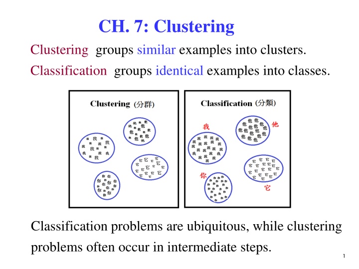
CH. 7: Clustering Clustering groups similar examples into clusters. Classification groups identical examples into classes. Classification problems are ubiquitous, while clustering problems often occur in intermediate steps. 1

7.1 Introduction Consider: Density Estimation Data points x { n } i i= 1 Density estimation Density distribution ( ) p x 2

Methods of density estimation: Parametric: The sample comes from a single known distribution model , e.g., . ( ) p x ( ) x : ( , ) p N = Parameters: { , } Semiparametric: The sample consists of many groups, each with a known distribution model. The distribution of data is a mixture of known distribution models, i.e., ( ) ( ) ( ) 1 i = { ( ), i i P C = Nonparametric: No distribution model is known. Parameters: { ( ), i P C = K Assume ( p x , }K i i = ) = x x | . | : ( , ) p P C p C C N i i i i i Parameters: 1 ( ) K x | } . i = p C 1 i 3

Clustering is an important step in determining #clusters in semiparametric and nonparametric estimations. 7.2 Hierarchical Clustering Cluster based on distances between instances Distance measure between instances xr and xs (1) Minkowski (Lp) (Euclidean for p = 2) ( M , d 1/ p ) ( ) p = r s r j s j x x d j x x = 1 (2) City-block distance ( CB d x x ) = r s r j s j d j , x x = 1 4

Distance between two groups Gi and Gj: ( ) ( ) = r s x x ( d ( x x d ) , c c i j , min G = , Single-link: d G G d i j r s x x max G ave x i G ) = , G i j ) ( ) = r s Complete-link: x x , , d G G ( i d G G i j ) r s x x , G ) i j r s , , Average-link: j ( r s x , G j ( , Centroid distance: d G G d i j c c i , : the centroids of Gi and Gj j 5

Approaches of clustering: (a) Agglomerative Clustering -- Start with N groups each with one instance and merge two closest groups at each iteration until there is a single one. (b) Divisive Clustering -- Start with a single group and dividing large group into two smaller groups, until each group contains a single instance. 6

Example: Single-Link Agglomerative Clustering Start with 6 groups each with one instance and merge two closest groups at each iteration until there is a single one. Next, select a threshold to get the clusters. 7

7.3 k-Means Clustering Given a sample and #clusters k, { } X = m t N t x = 1 find the centers , i = 1, .., k, of clusters. i 8

9

m Methods of initializing i 1) Randomly select k well separate examples as the m initial . i 2) Add to the mean m of data with k small random = + m m v vectors to get the initial . iv i i 3) Calculate the principal component, divide its range into k equal intervals, partition the data into k groups, take the means of these groups m as the initial . i 10

Measure of goodness of clustering: Xie-Beni index S: K N 2 x m m it t i overall average compactness separation = = = = 1 1 S i t 2 m m min i j N i j , Fukuyama-Sugeno index: Classification entropy index: 11

Fuzzy k-Means Clustering { } , = x t N t X Giving a set of data points = 1 K K N 2 = 1 subject to = x m Minimize c it t J it i = 1 i = = 1 1 i t K N N 2 = + x m c it t Minimize J f i t t = = = 1 1 1 i t t K = where 1 f t it = 1 i = N dJ d m = x m c it t 2 0, Let i = 1 t i = N N m x c it t c it / ----- (A) i = = 1 1 t t 12

= dJ d 2 + = x m 1 c it t 0 --- (B) c Let i t it 1 1/( 1) c 2 x m t k i = --- (C) it 2 x m t = 1 j j it according to (C) Steps: 1) Compute miaccording to (A) 2) Compute it by (C), it to obtain 3) Update it max{ i t } , stop 4) If it , = , go to step 2 otherwise it it 13

7.4 Semiparametric Density Estimation { } , = x t N t X the sample Given an unlabeled sample consists of many groups, each with a known distribution model. The distribution of data is a mixture of known distribution models, i.e., = 1 K K K ( ) ( i P C p ( p = ( | p x ) ( ) ( ) x = = = x ) ( ) P C ) i C : x | | , 1 p C p C i i i i = = = 1 1 1 i i i x | C where : cluster densities : mixture proportions i ( , ) i i N i i Assume . The model leads to the Gaussian mixture model. 14

= { , }K i i , : the parameters to be estimated = 1 i i Steps of semiparametric estimation: { } , = x t N t X Given an unlabeled sample = 1 1) Estimate the label of each example x e.g., K-means method 2) Estimate parameters of the mixture model e.g., EM algorithm 15

7.5 Expectation-Maximization Algorithm { } , = x t N t X Problem: Given an unlabeled sample = 1 = { , ( ) x }K estimate the parameters of a , = ( 1 i i i i K ) = x | p p C mixture Gaussian model , i i = 1 N i x ( | p ) : ( , ). C where K is known and i i i The problem involves two sets of random variables: X : observable variables examples of the sample Z : hidden variables - class labels of examples 16

The complete log-likelihood of the joint distribution of X and Z, = = t t t t x z x z ( | , ) log ( , | ) log ( , | ) L X Z p p c t t Method: Estimate by maximizing the available incomplete log-likelihood of unlabeled sample { } . = x t N t X = 1 = = t t x x ( | ) log ( | ) log ( | ) L X p p t t ) k = t x log ( | p C i i = 1 t i 17

The steps of finding the parameters : l = Let 0. 1. Estimate from sample X { , i i = , } l l l l i K i = 1 using k-means technique. 0 0 0 0 Estimate by applying k-means { , , }K i i i = = , 1 i 0 i 0 i 0 i i 1, , = , , to X and then calculate for n N K 0 clusters, where and is the number of i = in i examples in cluster i. = l l ( | , ) 2. Calculate c L L X Z c l = l l c cL [ ] Q E L Compute the expectation of over Z 18

+ 1 = l l argmax . 3. Find Q + 1 l l 4. Return if ; l otherwise go to step 2. + 1, = = + l l 1, l l EM algorithm: 0 Initialization: estimate = = l c l l l c ( | , ) and X Z [ ] L L Q E L E-step: compute c + 1 = l l M-step: compute argmax Q Terminate when + 1 l l 19

E-steps: Define indicator variables t x 1 0 if otherwise C = = t t t t K t k z ( , z z , , ), where i z z 1 2 z is a multinomial distribution of k classes ( ) 1 i i = = The likelihood of example K t t t p p C = The joint density ( x z p K K t i z t i z = = t ( ) z --- (A) P P C i i 1 tx K t i t i z z = = t x z x x ( | ) ( | ) ( ) --- (B) p i i = 1 1 i i = t t t t t x z ) ( ). --- (C) z P , ) ( | p The complete log-likelihood of the sample 20

( ) ( ) = t t x z | , log , | L X Z p c t | , ) ( x z t t t z = log ( | ) p P (C) t ( ) ( ) = + t t t x z z log | , log | p P t t K K t i t i z z + t x = log ( | ) log p i i (B)(A) = = 1 1 t i t i K K = + t i t t i x l og ( | ) log z p z i i = = 1 1 t i t i ( ) N K = + t i t x [log | log ] z p i i = = 1 1 t i 21

( ) | , cL X Z The expectation of over Z : ( ) = l l ( | ) [ | , | , ] Q E L X Z X c ( ) N K = + t i t x [log | log ] E z p i i = = 1 1 t i ( ) N K = + t i t l t l x x [ | , ][log | log ] E z p i i = = 1 1 t i = E z = + = t i t l t i t l t i t l x x x , 0 ( 0 , ) 1 ( 1 , ) P z P z t i : 0/1 z ( ) ( | ) = = t t i l t i l x | 1, 1| p z P z = = = t i t l x ( 1 , ) P z ( ) t l x p Bayes' rule 22

( p ) ( ) ) ( P C t l x | , p C P C ( ) i i = = = t l t x | , P C h ( ) i i t l x | , C Bayes' rule j j j ( ) = + l t i t l t l x x ( | ) [ | , ][log | log ] Q E z p t i i i ( ) = + t t l x [log | log ] h p t i i i i ( ) = + t t l t x log | log h p h t i t i i i i i 23

M-steps: (i) Estimating : i ( ) t t l x Q log | is independent of and h p t i i i i = 1. i i = + t Define log (1 ). J h t i i i i i = = t Solve for by letting / 0. / . J h N i i i i i (ii) Estimating , : i i ( ) t t x Q log is independent of | . h p G t i i i i = t t Define log ( | ). J h p x t i i i 24

( ) t l x m Q | : ( , ). p N S i i i + + + 1 1 1 = m l l i l Solve for ( , ) by letting iS = = = m / 0 and / 0, 1, , . K J J S i Get i i + + 1 1 t t t t l i t l i T x x m x m ( )( t i h ) h h + + 1 1 = = l i l m i i , , where S i h i i t i i i ( p ) ( ) ) ( P C t l x | , p C P C i i = t h ( ) i t l x | , C j j j 1/2 + + 1 1 1 exp[( 1/2)(( t l i m T t l i m x m x m ) ( ))] S S = i i S i 1/2 + + 1 1 1 exp[( 1/2)(( t l j T t l j x x ) ( ))] S j j j j 25

Summary of EM algorithm: X = , , { , x x x Given an unlabeled sample }, 1 2 N 0 0 i 0 i 0 i = }K 1. Estimate { , , = 1 i jx 2. E-step: Calculate for each data the probability p th jx of the Gaussian being responsible for k jk x ( | ) p C = k j k C p jk x K i = ( | ) p 1 i j i 3. M-step: Update the Gaussian parameters = new new k new k new k K k { , , } = 1 26

x N j p 1 N N = = new k 1 N j = new k ; p jk p j ; jk = 1 j = 1 jk new k new T k x x N j ( )( ) p = 1 = new k jk j j . N j p = 1 jk + 1 l l 4. Stop when 27

Summary Clustering groups similar examples into clusters. Classification groups identical examples into classes. Consider: Density Estimation Data points n { } i i= x 1 Density estimation Density distribut ion p x ( ) 28

Methods of density estimation: Parametric: The sample comes from a single known distribution model Semiparametric: The sample consists of many groups, each with a known distribution model. Nonparametric: No distribution model is known. Clustering plays an important role in semiparametric and nonparametric estimations. 29

Hierarchical Clustering (a) Agglomerative Clustering -- Start with N groups each with one instance and merge two closest groups at each iteration until there is a single one. (b) Divisive Clustering -- Start with a single group and dividing large group into two smaller groups, until each group contains a single instance. 30

k-Means Clustering Given a sample and #clusters k, { } x X = m t N t = 1 find the centers , i = 1, .., k, of clusters. i 31

Fuzzy k-Means Clustering { } , = x t N t X Giving a set of data points = 1 K K N 2 = 1 subject to = x m Minimize c it t J it i = 1 i = = 1 1 i t Steps: 1 1/( 1) c 2 x m t k i = 1) Compute it 2 x m t = 1 j j N N = m x c it t c it / 2) Compute i = = 1 1 t t it 3) Update 32

it max{ i t } , stop 4) If it , = go to step 2 , otherwise it it Measure of goodness of clustering: Xie-Beni index S, Fukuyama-Sugeno index, Classification entropy index 33

EM algorithm: Given an unlabeled sample X = , , { , x x x }, 1 2 N 1. Initialization: 0 0 0 0 Estimate by applying K-means { , , }K i i i = = 1 i 0 i 0 i 0 i i 1, , = , , , to X and calculate , for each n N K 0 cluster, where and is the number of i = i in data points in cluster i. p 2. E-step: Calculate for each data the probability jx jk of the Gaussian being responsible for k jx th 34

x ( | ) p C = k j k C p jk x K i = ( | ) p 1 i j i 3. M-step: Update the Gaussian parameters = new new k new k new k K k { , , } = 1 x N j p 1 N N = = new k 1 N j = new k ; p jk p j ; jk = 1 j = 1 jk new k new T k x x N j ( )( ) p = 1 = new k jk j j . N j p = 1 jk + 1 l l 4. Stop when 35